Interactive
- spb.interactive.iplot(*args, show=True, **kwargs)[source]
Create an interactive application containing widgets and charts in order to study symbolic expressions.
Note: this function is already integrated with many of the usual plotting functions: since their documentation is more specific, it is highly recommended to use those instead.
However, the following documentation explains in details the main features exposed by the interactive module, which might not be included on the documentation of those other functions.
- Parameters
- argstuples
Each tuple represents an expression. Depending on the type of expression, the tuple should have the following forms:
line: (expr, range, label [optional])
parametric line: (expr1, expr2, expr3 [optional], range, label [optional])
surface: (expr, range1, range2, label [optional])
parametric surface: (expr1, expr2, expr3, range1, range2, label [optional])
The label is always optional, whereas the ranges must always be specified. The ranges will create the discretized domain.
- paramsdict
A dictionary mapping the symbols to a parameter. The parameter can be:
an instance of param.parameterized.Parameter.
a tuple of the form: (default, min, max, N, tick_format, label, spacing) where:
- default, min, maxfloat
Default value, minimum value and maximum value of the slider, respectively. Must be finite numbers.
- Nint, optional
Number of steps of the slider.
- tick_formatTickFormatter or None, optional
Provide a formatter for the tick value of the slider. If None, panel will automatically apply a default formatter. Alternatively, an instance of bokeh.models.formatters.TickFormatter can be used. Default to None.
- label: str, optional
Custom text associated to the slider.
- spacingstr, optional
Specify the discretization spacing. Default to “linear”, can be changed to “log”.
Note that the parameters cannot be linked together (ie, one parameter cannot depend on another one).
- aspect(float, float) or str, optional
Set the aspect ratio of the plot. The value depends on the backend being used. Read that backend’s documentation to find out the possible values.
- backendPlot, optional
The backend to be used to generate the plot. It must be a subclass of spb.backends.base_backend.Plot. If not provided, the module will use the default backend.
- color_funccallable, optional
A numerical function which defines the 2D line color or the surface color:
For 2D plots, a function of two variables is needed: x, y (the points computed by the internal algorithm).
For 3D surfaces, a function of three variables is needed: x, y, z (the points computed by the internal algorithm).
For 3D parametric surfaces, a function of five variables is needed: x, y, z, u, v (the points computed by the internal algorithm and the parameters).
For surface plots, the coloring is applied only if
use_cm=True.- labellist/tuple, optional
The labels to be shown in the legend. If not provided, the string representation of expr will be used. The number of labels must be equal to the number of series generated by the plotting function.
- layoutstr, optional
The layout for the controls/plot. Possible values:
‘tb’: controls in the top bar.
‘bb’: controls in the bottom bar.
‘sbl’: controls in the left side bar.
‘sbr’: controls in the right side bar.
Default layout to ‘tb’. Note that side bar layouts may not work well with some backends.
- ncolsint, optional
Number of columns to lay out the widgets. Default to 2.
- is_complexboolean, optional
Default to False. If True, it directs the internal algorithm to create all the necessary series to create a complex plot (for example, one for the real part, one for the imaginary part).
- is_vectorboolean, optional
Default to False. If True, it directs the internal algorithm to create all the necessary series to create a vector plot (for example, plotting the magnitude of the vector field as a contour plot).
- namestr, optional
The name to be shown on top of the interactive application, when served on a new browser window. Refer to
servableto learn more. Default to an empty string.- pane_kwdict, optional
A dictionary of keyword/values which is passed to the pane containing the chart in order to further customize the output (read the Notes section to understand how the interactive plot is built). The following web pages shows the available options:
- rendering_kwdict or list of dicts, optional
A dictionary of keywords/values which is passed to the backend’s function to customize the appearance of lines, surfaces, etc. Refer to the plotting library (backend) manual for more informations. If a list of dictionaries is provided, the number of dictionaries must be equal to the number of series generated by the plotting function.
- servablebool, optional
Default to False, which will show the interactive application on the output cell of a Jupyter Notebook. If True, the application will be served on a new browser window.
- showbool, optional
Default to True. If True, it will return an object that will be rendered on the output cell of a Jupyter Notebook. If False, it returns an instance of InteractivePlot, which can later be be shown by calling the show() method.
- use_latexbool, optional
Default to True. If True, the latex representation of the symbols will be used in the labels of the parameter-controls. If False, the string representation will be used instead.
- detect_polesboolean
Chose whether to detect and correctly plot poles in line plots. Defaulto to False. To improve detection, increase the number of discretization points n and/or change the value of eps.
- epsfloat
An arbitrary small value used by the detect_poles algorithm. Default value to 0.1. Before changing this value, it is recommended to increase the number of discretization points.
- n1, n2, n3int, optional
Set the number of discretization points in the three directions, respectively.
- nint, optional
Set the number of discretization points on all directions. It overrides n1, n2, n3.
- ncint, optional
Number of discretization points for the contour plot when is_vector=True.
- throttledboolean, optional
Default to False. If True the recompute will be done at mouse-up event on sliders. If False, every slider tick will force a recompute.
- titlestr, optional
Title of the plot.
- xlabelstr, optional
Label for the x-axis.
- ylabelstr, optional
Label for the y-axis.
- zlabelstr, optional
Label for the z-axis.
- xlim(float, float), optional
Denotes the x-axis limits, (min, max).
- ylim(float, float), optional
Denotes the y-axis limits, (min, max).
- zlim(float, float), optional
Denotes the z-axis limits, (min, max).
See also
Notes
This function is specifically designed to work within Jupyter Notebook. It is also possible to use it from a regular Python console, by executing:
iplot(..., servable=True), which will create a server process loading the interactive plot on the browser. However,K3DBackendis not supported in this mode of operation.The interactive application generated by
iplotconsists of two main containers:a pane containing the widgets.
a pane containing the chart. We can further customize this container by setting the
pane_kwdictionary. Please, read its documentation to understand the available options.
Some examples use an instance of
PrintfTickFormatterto format the value shown by a slider. This class is exposed by Bokeh, but can be used byiplotwith any backend. Refer to 1 for more information about tick formatting.It has been observed that Dark Reader (or other night-mode-enabling browser extensions) might interfere with the correct behaviour of the output of
iplot. Please, consider addinglocalhostto the exclusion list of such browser extensions.Say we are creating two different interactive plots and capturing their output on two variables, using
show=False. For example,p1 = iplot(..., show=False)andp2 = iplot(..., show=False). Then, runningp1.show()on the screen will result in an error. This is standard behaviour that can’t be changed, as panel’s parameters are class attributes that gets deleted each time a new instance is created.MatplotlibBackendcan be used, but the resulting figure is just a PNG image without any interactive frame. Thus, data exploration is not great. Therefore, the use ofPlotlyBackendorBokehBackendis encouraged.Once this module has been loaded, there could be problems with all other plotting functions when using
BokehBackend, namely the figure won’t show up in the output cell. If that is the case, we might try to turn off automatic updates on panning by settingupdate_event=Falsein the function call.When
BokehBackendis used:the user-defined theme won’t be applied.
rendering of gradient lines is slow.
color bars might not update their ranges.
Once this module has been loaded and
iplothas been executed, the safest procedure to restart Jupyter Notebook’s kernel is the following:save the current notebook.
close the notebook and Jupyter server.
restart Jupyter server and open the notebook.
reload the cells.
Failing to follow this procedure might results in the notebook to become unresponsive once the module has been reloaded, with several errors appearing on the output cell.
References
Examples
NOTE: the following examples use the ordinary plotting function because
iplotis already integrated with them.Surface plot between -10 <= x, y <= 10 with a damping parameter varying from 0 to 1, with a default value of 0.15, discretized with 50 points on both directions. Note the use of threed=True to specify a 3D plot. If threed=False, a contour plot will be generated.
from sympy import (symbols, sqrt, cos, exp, sin, pi, re, im,
    Matrix, Plane, Polygon, I, log)
from spb import *
x, y, z = symbols("x, y, z")
r = sqrt(x**2 + y**2)
d = symbols('d')
expr = 10 * cos(r) * exp(-r * d)
plot3d(
    (expr, (x, -10, 10), (y, -10, 10)),
    params = { d: (0.15, 0, 1) },
    title = "My Title",
    xlabel = "x axis",
    ylabel = "y axis",
    zlabel = "z axis",
    backend = PB,
    n = 51,
    use_cm = True,
    use_latex=False,
    wireframe = True, wf_n1=15, wf_n2=15,
    wf_rendering_kw={"line_color": "#003428", "line_width": 0.75}
)
(Source code, small.png, large.png, html, pdf)

A line plot of the magnitude of a transfer function, illustrating the use of multiple expressions and:
some expression may not use all the parameters.
custom labeling of the expressions.
custom rendering of the expressions.
custom number of steps in the slider.
custom format of the value shown on the slider. This might be useful to correctly visualize very small or very big numbers.
custom labeling of the parameter-sliders.
from sympy import (symbols, sqrt, cos, exp, sin, pi, re, im,
    Matrix, Plane, Polygon, I, log)
from spb import *
from bokeh.models.formatters import PrintfTickFormatter
formatter = PrintfTickFormatter(format="%.3f")
kp, t, z, o = symbols("k_P, tau, zeta, omega")
G = kp / (I**2 * t**2 * o**2 + 2 * z * t * o * I + 1)
mod = lambda x: 20 * log(sqrt(re(x)**2 + im(x)**2), 10)
plot(
    (mod(G.subs(z, 0)), (o, 0.1, 100), "G(z=0)", {"line_dash": "dotted"}),
    (mod(G.subs(z, 1)), (o, 0.1, 100), "G(z=1)", {"line_dash": "dotted"}),
    (mod(G), (o, 0.1, 100), "G"),
    params = {
        kp: (1, 0, 3),
        t: (1, 0, 3),
        z: (0.2, 0, 1, 200, formatter, "z")
    },
    backend = BB,
    n = 2000,
    xscale = "log",
    xlabel = "Frequency, omega, [rad/s]",
    ylabel = "Magnitude [dB]",
    use_latex = False,
)
(Source code, small.png, large.png, html, pdf)

A line plot illustrating the Fouries series approximation of a saw tooth wave and:
custom format of the value shown on the slider.
creation of an integer spinner widget. This is achieved by setting
Noneas one of the bounds of the integer parameter.
from sympy import *
from spb import *
import param
from bokeh.models.formatters import PrintfTickFormatter

x, T, n, m = symbols("x, T, n, m")
sawtooth = frac(x / T)
# Fourier Series of a sawtooth wave
fs = S(1) / 2 - (1 / pi) * Sum(sin(2 * n * pi * x / T) / n, (n, 1, m))

formatter = PrintfTickFormatter(format="%.3f")
plot(
    (sawtooth, (x, 0, 10), "f", {"line_dash": "dotted"}),
    (fs, (x, 0, 10), "approx"),
    params = {
        T: (4, 0, 10, 80, formatter),
        m: param.Integer(4, bounds=(1, None), label="Sum up to n ")
    },
    xlabel = "x",
    ylabel = "y",
    backend = BB,
    use_latex = False
)
(Source code, small.png, large.png, html, pdf)

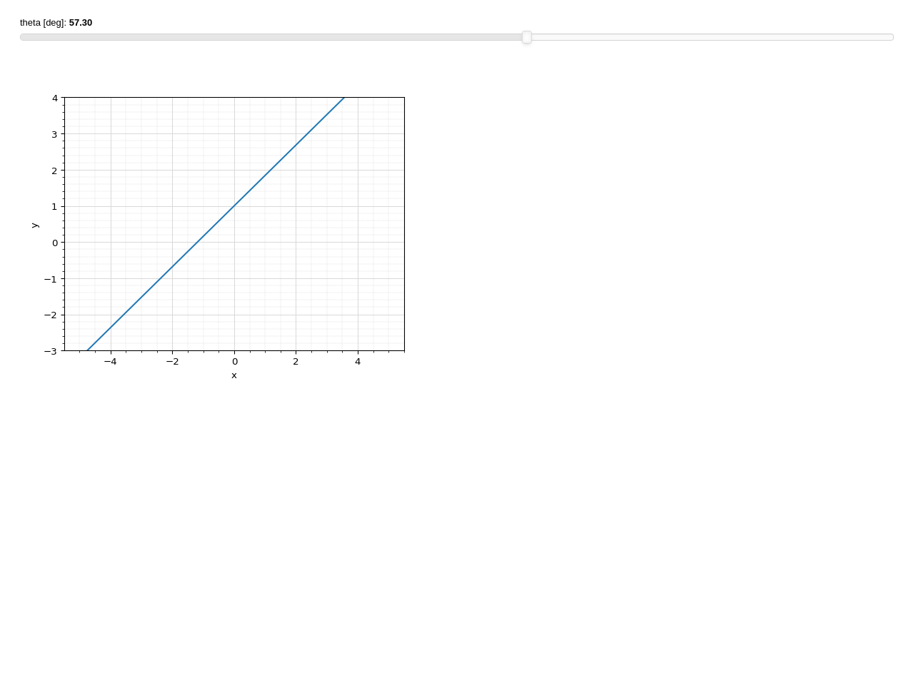
A line plot with a parameter representing an angle in radians, but showing the value in degrees on its label:
from sympy import sin, pi, symbols
from spb import *
from bokeh.models.formatters import FuncTickFormatter
# Javascript code is passed to `code=`
formatter = FuncTickFormatter(code="return (180./3.1415926 * tick).toFixed(2)")
x, t = symbols("x, t")

plot(
    (1 + x * sin(t), (x, -5, 5)),
    params = {
        t: (1, -2 * pi, 2 * pi, 100, formatter, "theta [deg]")
    },
    backend = MB,
    xlabel = "x", ylabel = "y",
    ylim = (-3, 4),
    use_latex = False,
)
(Source code, small.png, large.png, html, pdf)

Combine together InteractivePlot and
Plotinstances. The same parameters dictionary must be used for every interactive plot command. Note:the first plot dictates the labels, title and wheter to show the legend or not.
Instances of
Plotclass must be place on the right side of the + sign.show=False has been set in order for
iplotto return an instance ofInteractivePlot, which supports addition.Once we are done playing with parameters, we can access the backend with
p.backend. Then, we can use thep.backend.figattribute to retrieve the figure, orp.backend.save()to save the figure.
from sympy import sin, cos, symbols
from spb import *
x, u = symbols("x, u")
params = {
    u: (1, 0, 2)
}
p1 = plot(
    (cos(u * x), (x, -5, 5)),
    params = params,
    backend = MB,
    xlabel = "x1",
    ylabel = "y1",
    title = "title 1",
    legend = True,
    show = False,
    use_latex = False
)
p2 = plot(
    (sin(u * x), (x, -5, 5)),
    params = params,
    backend = MB,
    xlabel = "x2",
    ylabel = "y2",
    title = "title 2",
    show = False
)
p3 = plot(sin(x)*cos(x), (x, -5, 5), dict(marker="^"), backend=MB,
    adaptive=False, n=50,
    is_point=True, is_filled=True, show=False)
p = p1 + p2 + p3
p.show()
(Source code, small.png, large.png, html, pdf)

Serves the interactive plot to a separate browser window. Note that
K3DBackendis not supported for this operation mode. Also note the two ways to create a integer sliders.from sympy import * from spb import * import param from bokeh.models.formatters import PrintfTickFormatter formatter = PrintfTickFormatter(format='%.4f') p1, p2, t, r, c = symbols("p1, p2, t, r, c") phi = - (r * t + p1 * sin(c * r * t) + p2 * sin(2 * c * r * t)) phip = phi.diff(t) r1 = phip / (1 + phip) plot_polar( (r1, (t, 0, 2*pi)), params = { p1: (0.035, -0.035, 0.035, 50, formatter), p2: (0.005, -0.02, 0.02, 50, formatter), # integer parameter created with param r: param.Integer(2, softbounds=(2, 5), label="r"), # integer parameter created with usual syntax c: (3, 1, 5, 4) }, use_latex = False, backend = BB, aspect = "equal", n = 5000, layout = "sbl", ncols = 1, servable = True, name = "Non Circular Planetary Drive - Ring Profile" )
(Source code, small.png, large.png, html, pdf)

- spb.interactive.create_series(*args, **kwargs)[source]
Create interactive data series, ie. series whose numerical data depends on the expression and all its parameters.
Typical usage examples are in the followings:
- Create a single interactive series:
create_series([expr, range], **kwargs)
- Create multiple interactive series:
create_series([(expr1, range1), (expr2, range2)], **kwargs)
The correct series type is instantiated only if all ranges are specified. So, to create an interactive line series, one range must be specified. To create an interactive surface series, two ranges must be provided, and so on.
- Parameters
- argslist/tuple
A list or tuple of the form
[(expr1, range1), ...], where:- exprExpr
Expression (or expressions) representing the function to evaluate.
- range: (symbol, min, max)
A 3-tuple (or multiple 3-tuple) denoting the range of the variable. For the function to work properly, all ranges must be provided.
- paramsdict
A dictionary mapping symbols to numerical values. If not specified,
iplotshould be provided instead.- iplotInteractivePlot, optional
An existing instance of
InteractivePlotfrom which the parameters will be extracted. If bothparamsandiplotare provided, theniplothas the precedence.- is_complexboolean, optional
Default to False. If True, it directs the internal algorithm to create all the necessary series to create a complex plot (for example, one for the real part, one for the imaginary part, …).
- is_polarboolean, optional
Default to False. If True:
for a 2D line plot requests the backend to use a polar chart.
for a 3D surface (or contour) requests a polar discretization. In this case, the first range represents the radius, the second one represents the angle.
- is_vectorboolean, optional
Default to False. If True, it directs the internal algorithm to create all the necessary series to create a vector plot (for example, plotting the magnitude of the vector field as a contour plot, …).
- n1, n2, n3int, optional
Number of discretization points in the 3 directions.
- nint, optional
Set the same number of discretization points on all directions.
- Returns
- slist
A list of interactive data series.
See also
Notes
The keyword arguments to be provided depends on the interested data series to be created. For example, if we are trying to plot a line, then the same keyword argument associated to the
plot()function can be used. Similarly, if we are trying to create vector-related interactive series, the same keyword arguments associated toplot_vector()can be used. And so on.However, interactive data series do not support adaptive algorithms. Hence, adaptive-related keyword arguments will not be used.
Examples
>>> from sympy import (symbols, pi, sin, cos, exp, Plane,
...     Matrix, gamma, I, sqrt, Abs)
>>> from spb.interactive import create_series
>>> u, v, x, y, z = symbols('u, v, x:z')
2D line interactive series:
>>> s = create_series((u * sqrt(x), (x, -5, 5)), params={u: 1})
>>> print(len(s), type(s[0]))
(1, spb.series.LineInteractiveSeries)
2D parametric line interactive series:
>>> s = create_series((u * cos(x), u * sin(x), (x, -5, 5)), params={u: 1})
>>> len(s), type(s[0])
(1, spb.series.Parametric2DLineInteractiveSeries)
Multiple 2D lines interactive series:
>>> s = create_series(
...     (u * sqrt(x), (x, -5, 5)),
...     (cos(u * x), (x, -3, 3)),
...     params={u: 1})
>>> len(s), type(s[0]), type(s[1])
(2, spb.series.LineInteractiveSeries, spb.series.LineInteractiveSeries)
Surface interactive series:
>>> s = create_series((cos(x**2 + u * y**2), (x, -5, 5), (y, -5, 5)),
...     params={u: 1}, threed=True)
>>> len(s), type(s[0])
(1, spb.series.SurfaceInteractiveSeries)
Contour interactive series:
>>> s = create_series((cos(x**2 + u * y**2), (x, -5, 5), (y, -5, 5)),
...     params={u: 1}, threed=False)
>>> len(s), type(s[0])
(1, spb.series.ContourInteractiveSeries)
Interactive series of the absolute value of a complex function colored by its argument over a real domain. Note that we are passing
is_complex=True:>>> s = create_series((u * sqrt(x), (x, -5, 5)), params={u: 1}, ... is_complex=True) >>> len(s), type(s[0]) (1, spb.series.AbsArgLineInteractiveSeries)
Real and imaginary parts of a complex function over a real domain:
>>> s = create_series((u * sqrt(x), (x, -5, 5)), params={u: 1},
...     is_complex=True, absarg=False, real=True, imag=True)
>>> len(s), type(s[0]), type(s[1])
(2, spb.series.LineInteractiveSeries, spb.series.LineInteractiveSeries)
Complex domain coloring interactive series:
>>> s = create_series((u * sqrt(x), (x, -5-5j, 5+5j)), params={u: 1},
...     is_complex=True)
>>> len(s), type(s[0])
Real and imaginary parts of a complex function over a complex domain:
>>> s = create_series((u * sqrt(x), (x, -5-5j, 5+5j)), params={u: 1},
...     is_complex=True, threed=True, absarg=False, real=True, imag=True)
>>> len(s), type(s[0]), type(s[1])
(2, spb.series.ComplexSurfaceInteractiveSeries, spb.series.ComplexSurfaceInteractiveSeries)
2D vector interactive series (only quivers):
>>> from sympy.vector import CoordSys3D
>>> N = CoordSys3D("N")
>>> i, j, k = N.base_vectors()
>>> x, y, z = N.base_scalars()
>>> a, b, c = symbols("a:c")
>>> v1 = -a * sin(y) * i + b * cos(x) * j
>>> s = create_series((v1, (x, -5, 5), (y, -4, 4)),
...     params={a: 2, b: 3}, is_vector=False)
>>> len(s), type(s[0])
(1, spb.series.Vector2DInteractiveSeries)
2D vector interactive series (contour + quivers):
>>> s = create_series((v1, (x, -5, 5), (y, -4, 4)),
...     params={a: 2, b: 3}, is_vector=True)
>>> len(s), type(s[0]), type(s[1])
(2, spb.series.ContourInteractiveSeries, spb.series.Vector2DInteractiveSeries)
Sliced 3D vector (single slice):
>>> from sympy import Plane
>>> v3 = a * z * i + b * y * j + c * x * k
>>> s = create_series((v3, (x, -5, 5), (y, -4, 4), (z, -6, 6)),
...     params={a: 2, b: 3, c: 1}, slice=Plane((1, 2, 3), (1, 0, 0)))
>>> len(s), type(s[0])
(1, spb.series.SliceVector3DInteractiveSeries)
Geometry interactive series:
>>> from sympy import Circle
>>> s = create_series((Circle((0, 0), u), ), params={u: 1})
>>> len(s), type(s[0])
(1, spb.series.GeometryInteractiveSeries)
- spb.interactive.create_widgets(params, **kwargs)[source]
Create panel’s widgets starting from parameters.
- Parameters
- paramsdict
A dictionary mapping the symbols to a parameter. The parameter can be:
an instance of param.parameterized.Parameter. Refer to 4 for a list of available parameters.
a tuple of the form: (default, min, max, N, tick_format, label, spacing) where:
- default, min, maxfloat
Default value, minimum value and maximum value of the slider, respectively. Must be finite numbers.
- Nint, optional
Number of steps of the slider.
- tick_formatTickFormatter or None, optional
Provide a formatter for the tick value of the slider. If None, panel will automatically apply a default formatter. Alternatively, an instance of bokeh.models.formatters.TickFormatter can be used. Default to None.
- label: str, optional
Custom text associated to the slider.
- spacingstr, optional
Specify the discretization spacing. Default to “linear”, can be changed to “log”.
Note that the parameters cannot be linked together (ie, one parameter cannot depend on another one).
- use_latexbool, optional
Default to True. If True, the latex representation of the symbols will be used in the labels of the parameter-controls. If False, the string representation will be used instead.
- Returns
- widgetsdict
A dictionary mapping the symbols from params to the appropriate widget.
See also
References
Examples
from sympy.abc import x, y, z
from spb.interactive import create_widgets
import param
from bokeh.models.formatters import PrintfTickFormatter
formatter = PrintfTickFormatter(format="%.4f")
r = create_widgets({
    x: (0.035, -0.035, 0.035, 100, formatter),
    y: (200, 1, 1000, 10, None, "test", "log"),
    z: param.Integer(3, softbounds=(3, 10), label="n")
})