Interactive

This module allows the creation of interactive widgets plots using either one of the following modules:

ipywidgets and ipympl: it probably has less dependencies to install and it might be a little bit faster at updating the visualization. However, it only works inside Jupyter Notebook.
Holoviz’s panel: works on any Python interpreter, as long as a browser is installed on the system. The interactive plot can be visualized directly in Jupyter Notebook, or in a new browser window where the plot can use the entire screen space. This might be useful to visualize plots with many parameters, or to focus the attention only on the plot rather than the code.

If only a minimal installation of this plotting module has been performed, then users have to manually install the chosen interactive modules.

By default, this plotting module will attempt to create interactive widgets with ipywidgets. To change interactive module, users can either:

specify the following keyword argument to use Holoviz’s Panel: imodule="panel". Alternatively, specify imodule="ipywidgets" to use ipywidgets.
Modify the configuration file to permanently change the interactive module. More information are provided in 4 - Customizing the module.

Note that:

interactive capabilities are already integrated with many plotting functions. The purpose of the following documentation is to show a few more examples for each interactive module.
if user is attempting to execute an interactive widget plot and gets an error similar to the following: TraitError: The ‘children’ trait of a Box instance contains an Instance of a TypedTuple which expected a Widget, not the FigureCanvasAgg at ‘0x…’. It means that the ipywidget module is being used with Matplotlib, but the interactive Matplotlib backend has not been loaded. First, execute the magic command %matplotlib widget, then execute the plot command.
For technical reasons, all interactive-widgets plots in this documentation are created using Holoviz’s Panel. Often, they will ran just fine with ipywidgets too. However, if a specific example uses the param library, then users will have to modify the params dictionary in order to make it work with ipywidgets. A couple of examples are provided below.

The prange class

class spb.utils.prange(*args)[source]

Represents a plot range, an entity describing what interval a particular variable is allowed to vary. It is a 3-elements tuple: (symbol, minimum, maximum).

Notes

Why does the plotting module needs this class instead of providing a plotting range with ordinary tuple/list? After all, ordinary plots works just fine.

If a plotting range is provided with a 3-elements tuple/list, the internal algorithm looks at the tuple and tries to determine what it is. If minimum and maximum are numeric values, than it is a plotting range.

Hovewer, there are some plotting functions in which the expression consists of 3-elements tuple/list. The plotting module is also interactive, meaning that minimum and maximum can also be expressions containing parameters. In these cases, the plotting range is indistinguishable from a 3-elements tuple describing an expression.

This class is meant to solve that ambiguity: it only represents a plotting range.

Examples

Let x be a symbol and u, v, t be parameters. An example plotting range is:

>>> from sympy import symbols
>>> from spb import prange
>>> x, u, v, t = symbols("x, u, v, t")
>>> prange(x, u * v, v**2 + t)
(x, u*v, t + v**2)

Holoviz’s panel

spb.interactive.panel.iplot(*series, show=True, **kwargs)[source]

Create an interactive application containing widgets and charts in order to study symbolic expressions, using Holoviz’s Panel for the user interace.

Note: this function is already integrated with many of the usual plotting functions: since their documentation is more specific, it is highly recommended to use those instead.

However, the following documentation explains in details the main features exposed by the interactive module, which might not be included on the documentation of those other functions.

Parameters:

seriesBaseSeries

Instances of BaseSeries, representing the symbolic expression to be plotted.

paramsdict

A dictionary mapping the symbols to a parameter. The parameter can be:

an instance of param.parameterized.Parameter.
a tuple of the form: (default, min, max, N, tick_format, label, spacing) where:
- default, min, maxfloat
  Default value, minimum value and maximum value of the slider, respectively. Must be finite numbers.
- Nint, optional
  Number of steps of the slider.
- tick_formatTickFormatter or None, optional
  Provide a formatter for the tick value of the slider. If None, panel will automatically apply a default formatter. Alternatively, an instance of bokeh.models.formatters.TickFormatter can be used. Default to None.
- label: str, optional
  Custom text associated to the slider.
- spacingstr, optional
  Specify the discretization spacing. Default to "linear", can be changed to "log".

Note that the parameters cannot be linked together (ie, one parameter cannot depend on another one).

layoutstr, optional

The layout for the controls/plot. Possible values:

'tb': controls in the top bar.
'bb': controls in the bottom bar.
'sbl': controls in the left side bar.
'sbr': controls in the right side bar.

If servable=False (plot shown inside Jupyter Notebook), then the default value is 'tb'. If servable=True (plot shown on a new browser window) then the default value is 'sbl'. Note that side bar layouts may not work well with some backends.

ncolsint, optional

Number of columns to lay out the widgets. Default to 2.

namestr, optional

The name to be shown on top of the interactive application, when served on a new browser window. Refer to servable to learn more. Default to an empty string.

pane_kwdict, optional

A dictionary of keyword/values which is passed to the pane containing the chart in order to further customize the output (read the Notes section to understand how the interactive plot is built). The following web pages shows the available options:

Refer to [2] for MatplotlibBackend. Two interesting options are:
- interactive: wheter to activate the ipympl interactive backend.
- dpi: set the dots per inch of the output png. Default to 96.
Refer to [3] for PlotlyBackend.

servablebool, optional

Default to False, which will show the interactive application on the output cell of a Jupyter Notebook. If True, the application will be served on a new browser window.

showbool, optional

Default to True. If True, it will return an object that will be rendered on the output cell of a Jupyter Notebook. If False, it returns an instance of InteractivePlot, which can later be be shown by calling the show() method.

templateoptional

Specify the template to be used to build the interactive application when servable=True. It can be one of the following options:

None: the default template will be used.
dictionary of keyword arguments to customize the default template. Among the options:
- full_width (boolean): use the full width of the browser page. Default to True.
- sidebar_width (str): CSS value of the width of the sidebar in pixel or %. Applicable only when layout='sbl' or layout='sbr'.
- show_header (boolean): wheter to show the header of the application. Default to True.
an instance of pn.template.base.BasicTemplate
a subclass of pn.template.base.BasicTemplate

throttledboolean, optional

Default to False. If True the recompute will be done at mouse-up event on sliders. If False, every slider tick will force a recompute.

use_latexbool, optional

Default to True. If True, the latex representation of the symbols will be used in the labels of the parameter-controls. If False, the string representation will be used instead.

See also

create_widgets

Notes

This function is specifically designed to work within Jupyter Notebook. It is also possible to use it from a regular Python console, by executing: iplot(..., servable=True), which will create a server process loading the interactive plot on the browser. However, K3DBackend is not supported in this mode of operation.
The interactive application generated by iplot consists of two main containers:
- a pane containing the widgets.
- a pane containing the chart. We can further customize this container by setting the pane_kw dictionary. Please, read its documentation to understand the available options.
Some examples use an instance of PrintfTickFormatter to format the value shown by a slider. This class is exposed by Bokeh, but can be used by iplot with any backend. Refer to [1] for more information about tick formatting.
It has been observed that Dark Reader (or other night-mode-enabling browser extensions) might interfere with the correct behaviour of the output of iplot. Please, consider adding localhost to the exclusion list of such browser extensions.
Say we are creating two different interactive plots and capturing their output on two variables, using show=False. For example, p1 = iplot(..., show=False) and p2 = iplot(..., show=False). Then, running p1.show() on the screen will result in an error. This is standard behaviour that can’t be changed, as panel’s parameters are class attributes that gets deleted each time a new instance is created.
MatplotlibBackend can be used, but the resulting figure is just a PNG image without any interactive frame. Thus, data exploration is not great. Therefore, the use of PlotlyBackend or BokehBackend is encouraged.
When BokehBackend is used:
- the user-defined theme won’t be applied.
- rendering of gradient lines is slow.
- color bars might not update their ranges.

8. Once this module has been loaded and executed, the safest procedure to restart Jupyter Notebook’s kernel is the following:

save the current notebook.

close the notebook and Jupyter server.

restart Jupyter server and open the notebook.

reload the cells.

Failing to follow this procedure might results in the notebook to become unresponsive once the module has been reloaded, with several errors appearing on the output cell.

References

Examples

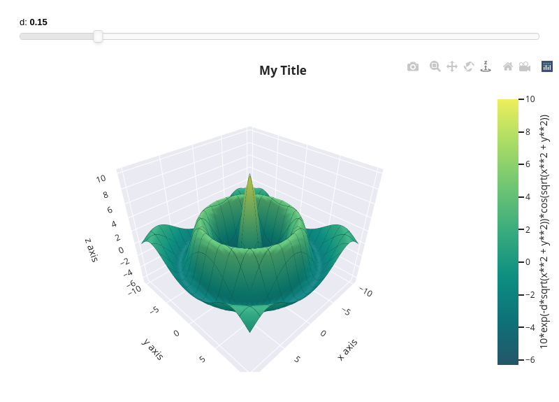
NOTE: the following examples use the ordinary plotting function because iplot is already integrated with them.

Surface plot between -10 <= x, y <= 10 with a damping parameter varying from 0 to 1, with a default value of 0.15, discretized with 50 points on both directions.

from sympy import (symbols, sqrt, cos, exp, sin, pi, re, im,
    Matrix, Plane, Polygon, I, log)
from spb import *
x, y, z = symbols("x, y, z")
r = sqrt(x**2 + y**2)
d = symbols('d')
expr = 10 * cos(r) * exp(-r * d)
plot3d(
    (expr, (x, -10, 10), (y, -10, 10)),
    params = { d: (0.15, 0, 1) },
    title = "My Title",
    xlabel = "x axis",
    ylabel = "y axis",
    zlabel = "z axis",
    backend = PB,
    n = 51,
    use_cm = True,
    use_latex=False,
    wireframe = True, wf_n1=15, wf_n2=15,
    wf_rendering_kw={"line_color": "#003428", "line_width": 0.75}
)

(Source code, small.png)

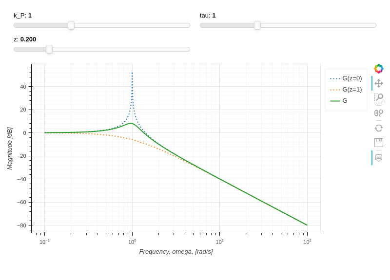
A line plot of the magnitude of a transfer function, illustrating the use of multiple expressions and:

some expression may not use all the parameters.
custom labeling of the expressions.
custom rendering of the expressions.
custom number of steps in the slider.
custom format of the value shown on the slider. This might be useful to correctly visualize very small or very big numbers.
custom labeling of the parameter-sliders.

from sympy import (symbols, sqrt, cos, exp, sin, pi, re, im,
    Matrix, Plane, Polygon, I, log)
from spb import *
from bokeh.models.formatters import PrintfTickFormatter
formatter = PrintfTickFormatter(format="%.3f")
kp, t, z, o = symbols("k_P, tau, zeta, omega")
G = kp / (I**2 * t**2 * o**2 + 2 * z * t * o * I + 1)
mod = lambda x: 20 * log(sqrt(re(x)**2 + im(x)**2), 10)
plot(
    (mod(G.subs(z, 0)), (o, 0.1, 100), "G(z=0)", {"line_dash": "dotted"}),
    (mod(G.subs(z, 1)), (o, 0.1, 100), "G(z=1)", {"line_dash": "dotted"}),
    (mod(G), (o, 0.1, 100), "G"),
    params = {
        kp: (1, 0, 3),
        t: (1, 0, 3),
        z: (0.2, 0, 1, 200, formatter, "z")
    },
    backend = BB,
    n = 2000,
    xscale = "log",
    xlabel = "Frequency, omega, [rad/s]",
    ylabel = "Magnitude [dB]",
    use_latex = False,
)

(Source code, small.png)

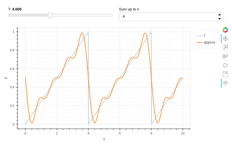
A line plot illustrating the Fouries series approximation of a saw tooth wave and:

custom format of the value shown on the slider.
creation of an integer spinner widget. This is achieved by setting None as one of the bounds of the integer parameter.

from sympy import *
from spb import *
import param
from bokeh.models.formatters import PrintfTickFormatter

x, T, n, m = symbols("x, T, n, m")
sawtooth = frac(x / T)
# Fourier Series of a sawtooth wave
fs = S(1) / 2 - (1 / pi) * Sum(sin(2 * n * pi * x / T) / n, (n, 1, m))

formatter = PrintfTickFormatter(format="%.3f")
plot(
    (sawtooth, (x, 0, 10), "f", {"line_dash": "dotted"}),
    (fs, (x, 0, 10), "approx"),
    params = {
        T: (4, 0, 10, 80, formatter),
        m: param.Integer(4, bounds=(1, None), label="Sum up to n ")
    },
    xlabel = "x",
    ylabel = "y",
    backend = BB,
    use_latex = False
)

(Source code, small.png)

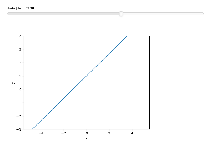
A line plot with a parameter representing an angle in radians, but showing the value in degrees on its label:

from sympy import sin, pi, symbols
from spb import *
from bokeh.models.formatters import FuncTickFormatter
# Javascript code is passed to `code=`
formatter = FuncTickFormatter(code="return (180./3.1415926 * tick).toFixed(2)")
x, t = symbols("x, t")

plot(
    (1 + x * sin(t), (x, -5, 5)),
    params = {
        t: (1, -2 * pi, 2 * pi, 100, formatter, "theta [deg]")
    },
    backend = MB,
    xlabel = "x", ylabel = "y",
    ylim = (-3, 4),
    use_latex = False,
)

(Source code, small.png)

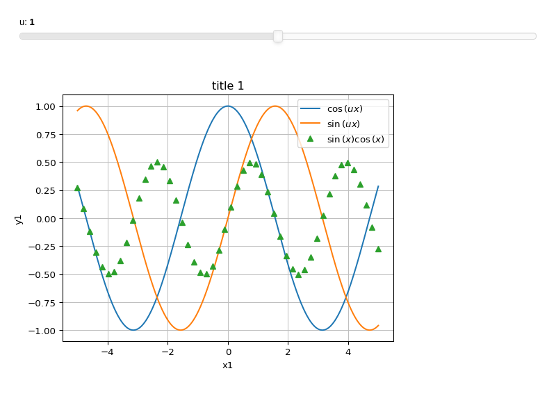
Combine together InteractivePlot and Plot instances. The same parameters dictionary must be used for every interactive plot command. Note:

the first plot dictates the labels, title and wheter to show the legend or not.
Instances of Plot class must be place on the right side of the + sign.
show=False has been set in order for iplot to return an instance of InteractivePlot, which supports addition.
Once we are done playing with parameters, we can access the backend with p.backend. Then, we can use the p.backend.fig attribute to retrieve the figure, or p.backend.save() to save the figure.

from sympy import sin, cos, symbols
from spb import *
x, u = symbols("x, u")
params = {
    u: (1, 0, 2)
}
p1 = plot(
    (cos(u * x), (x, -5, 5)),
    params = params,
    backend = MB,
    xlabel = "x1",
    ylabel = "y1",
    title = "title 1",
    legend = True,
    show = False,
    use_latex = False,
    imodule="panel"
)
p2 = plot(
    (sin(u * x), (x, -5, 5)),
    params = params,
    backend = MB,
    xlabel = "x2",
    ylabel = "y2",
    title = "title 2",
    show = False,
    imodule="panel"
)
p3 = plot(sin(x)*cos(x), (x, -5, 5), dict(marker="^"), backend=MB,
    adaptive=False, n=50,
    is_point=True, is_filled=True, show=False)
p = p1 + p2 + p3
p.show()

(Source code, small.png)

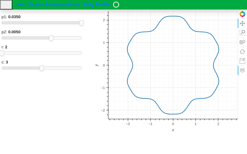
Serves the interactive plot to a separate browser window. Note that K3DBackend is not supported for this operation mode. Also note the two ways to create a integer sliders.

from sympy import *
from spb import *
import param
from bokeh.models.formatters import PrintfTickFormatter
formatter = PrintfTickFormatter(format='%.4f')

p1, p2, t, r, c = symbols("p1, p2, t, r, c")
phi = - (r * t + p1 * sin(c * r * t) + p2 * sin(2 * c * r * t))
phip = phi.diff(t)
r1 = phip / (1 + phip)

plot_polar(
    (r1, (t, 0, 2*pi)),
    params = {
        p1: (0.035, -0.035, 0.035, 50, formatter),
        p2: (0.005, -0.02, 0.02, 50, formatter),
        # integer parameter created with param
        r: param.Integer(2, softbounds=(2, 5), label="r"),
        # integer parameter created with usual syntax
        c: (3, 1, 5, 4)
    },
    use_latex = False,
    backend = BB,
    aspect = "equal",
    n = 5000,
    layout = "sbl",
    ncols = 1,
    servable = True,
    name = "Non Circular Planetary Drive - Ring Profile"
)

(Source code, small.png)

ipywidgets

spb.interactive.ipywidgets.iplot(*series, show=True, **kwargs)[source]

Create an interactive application containing widgets and charts in order to study symbolic expressions, using ipywidgets.

Note: this function is already integrated with many of the usual plotting functions: since their documentation is more specific, it is highly recommended to use those instead.

However, the following documentation explains in details the main features exposed by the interactive module, which might not be included on the documentation of those other functions.

Parameters:

seriesBaseSeries

Instances of BaseSeries, representing the symbolic expression to be plotted.

paramsdict

A dictionary mapping the symbols to a parameter. The parameter can be:

a widget.
a tuple of the form: (default, min, max, N, tick_format, label, spacing) where:
- default, min, maxfloat
  Default value, minimum value and maximum value of the slider, respectively. Must be finite numbers.
- Nint, optional
  Number of steps of the slider.
- label: str, optional
  Custom text associated to the slider.
- spacingstr, optional
  Specify the discretization spacing. Default to "linear", can be changed to "log".

Note that the parameters cannot be linked together (ie, one parameter cannot depend on another one).

layoutstr, optional

The layout for the controls/plot. Possible values:

'tb': controls in the top bar.
'bb': controls in the bottom bar.
'sbl': controls in the left side bar.
'sbr': controls in the right side bar.

The default value is 'tb'.

ncolsint, optional

Number of columns to lay out the widgets. Default to 2.

showbool, optional

Default to True. If True, it will return an object that will be rendered on the output cell of a Jupyter Notebook. If False, it returns an instance of InteractivePlot, which can later be be shown by calling the show() method.

use_latexbool, optional

Default to True. If True, the latex representation of the symbols will be used in the labels of the parameter-controls. If False, the string representation will be used instead.

Notes

This function is specifically designed to work within Jupyter Notebook and requires the ipywidgets module [4] .
To update Matplotlib plots, the %matplotlib widget command must be executed at the top of the Jupyter Notebook. It requires the installation of the ipympl module [5] .

References

Examples

NOTE: the following examples use the ordinary plotting function because iplot is already integrated with them.

Surface plot between -10 <= x, y <= 10 with a damping parameter varying from 0 to 1, with a default value of 0.15, discretized with 50 points on both directions.

from sympy import (symbols, sqrt, cos, exp, sin, pi, re, im,
    Matrix, Plane, Polygon, I, log)
from spb import *
x, y, z = symbols("x, y, z")
r = sqrt(x**2 + y**2)
d = symbols('d')
expr = 10 * cos(r) * exp(-r * d)
plot3d(
    (expr, (x, -10, 10), (y, -10, 10)),
    params = { d: (0.15, 0, 1) },
    title = "My Title",
    xlabel = "x axis",
    ylabel = "y axis",
    zlabel = "z axis",
    backend = PB,
    n = 51,
    use_cm = True,
    use_latex=False,
    wireframe = True, wf_n1=15, wf_n2=15,
    wf_rendering_kw={"line_color": "#003428", "line_width": 0.75}
)

A line plot illustrating how to specify widgets. In particular:

the parameter d will be rendered as a slider.
the parameter n is a spinner.
the parameter phi will be rendered as a slider: note the custom number of steps and the custom label.
when using Matplotlib, the %matplotlib widget must be executed at the top of the notebook.

%matplotlib widget
from sympy import *
from spb import *
import ipywidgets

x, phi, n, d = symbols("x, phi, n, d")
plot(
    cos(x * n - phi) * exp(-abs(x) * d), (x, -5*pi, 5*pi),
    params={
        d: (0.1, 0, 1),
        n: ipywidgets.BoundedIntText(value=2, min=1, max=10, description="$n$"),
        phi: (0, 0, 2*pi, 50, "$\phi$ [rad]")
    },
    ylim=(-1.25, 1.25))

A line plot illustrating the Fouries series approximation of a saw tooth wave and:

custom number of steps and label in the slider.
creation of an integer spinner widget.

from sympy import *
from spb import *
import ipywidgets

x, T, n, m = symbols("x, T, n, m")
sawtooth = frac(x / T)
# Fourier Series of a sawtooth wave
fs = S(1) / 2 - (1 / pi) * Sum(sin(2 * n * pi * x / T) / n, (n, 1, m))

formatter = PrintfTickFormatter(format="%.3f")
plot(
    (sawtooth, (x, 0, 10), "f", {"line_dash": "dotted"}),
    (fs, (x, 0, 10), "approx"),
    params = {
        T: (4, 0, 10, 80, "Period, T"),
        m: ipywidgets.BoundedIntText(value=4, min=1, max=100, description="Sum up to n ")
    },
    xlabel = "x",
    ylabel = "y",
    backend = BB
)

A line plot of the magnitude of a transfer function, illustrating the use of multiple expressions and:

some expression may not use all the parameters.
custom labeling of the expressions.
custom rendering of the expressions.
custom number of steps in the slider.
custom labeling of the parameter-sliders.

from sympy import (symbols, sqrt, cos, exp, sin, pi, re, im,
    Matrix, Plane, Polygon, I, log)
from spb import *
kp, t, z, o = symbols("k_P, tau, zeta, omega")
G = kp / (I**2 * t**2 * o**2 + 2 * z * t * o * I + 1)
mod = lambda x: 20 * log(sqrt(re(x)**2 + im(x)**2), 10)
plot(
    (mod(G.subs(z, 0)), (o, 0.1, 100), "G(z=0)", {"line_dash": "dotted"}),
    (mod(G.subs(z, 1)), (o, 0.1, 100), "G(z=1)", {"line_dash": "dotted"}),
    (mod(G), (o, 0.1, 100), "G"),
    params = {
        kp: (1, 0, 3),
        t: (1, 0, 3),
        z: (0.2, 0, 1, 200, "z")
    },
    backend = BB,
    n = 2000,
    xscale = "log",
    xlabel = "Frequency, omega, [rad/s]",
    ylabel = "Magnitude [dB]",
    use_latex = True,
)

A polar line plot. Note:

when using Matplotlib, the %matplotlib widget must be executed at the top of the notebook.
the two ways to create a integer sliders.

%matplotlib widget
from sympy import *
from spb import *
import ipywidgets

p1, p2, t, r, c = symbols("p1, p2, t, r, c")
phi = - (r * t + p1 * sin(c * r * t) + p2 * sin(2 * c * r * t))
phip = phi.diff(t)
r1 = phip / (1 + phip)

plot_polar(
    (r1, (t, 0, 2*pi)),
    params = {
        p1: (0.035, -0.035, 0.035, 50),
        p2: (0.005, -0.02, 0.02, 50),
        # integer parameter created with ipywidgets
        r: ipywidgets.BoundedIntText(value=2, min=2, max=5, description="r"),
        # integer parameter created with usual syntax
        c: (3, 1, 5, 4)
    },
    backend = MB,
    aspect = "equal",
    n = 5000,
    name = "Non Circular Planetary Drive - Ring Profile"
)

Combine together InteractivePlot and Plot instances. The same parameters dictionary must be used for every interactive plot command. Note:

the first plot dictates the labels, title and wheter to show the legend or not.
Instances of Plot class must be place on the right side of the + sign.
show=False has been set in order for iplot to return an instance of InteractivePlot, which supports addition.
Once we are done playing with parameters, we can access the backend with p.backend. Then, we can use the p.backend.fig attribute to retrieve the figure, or p.backend.save() to save the figure.

from sympy import sin, cos, symbols
from spb import *
x, u = symbols("x, u")
params = {
    u: (1, 0, 2)
}
p1 = plot(
    (cos(u * x), (x, -5, 5)),
    params = params,
    backend = MB,
    xlabel = "x1",
    ylabel = "y1",
    title = "title 1",
    legend = True,
    show = False
)
p2 = plot(
    (sin(u * x), (x, -5, 5)),
    params = params,
    backend = MB,
    xlabel = "x2",
    ylabel = "y2",
    title = "title 2",
    show = False
)
p3 = plot(sin(x)*cos(x), (x, -5, 5), dict(marker="^"), backend=MB,
    adaptive=False, n=50,
    is_point=True, is_filled=True, show=False)
p = p1 + p2 + p3
p.show()