Overview

The following overview briefly introduce the functionalities exposed by this module.

Plotting functions

The following functions are exposed by this module:

plot: visualize a function of a single variable, with the capability to correctly visualize discontinuities.
plot_piecewise: plot piecewise expressions, with the capability to correctly visualize discontinuities.
plot_polar: visualize a curve of a given radius as a function of an angle.
plot_list: visualize numerical data.
plot_parametric: visualize a 2D parametric curve.
plot_contour: visualized filled or line contours of a function of two variables.
plot3d: visualize a function of two variables.
plot3d_parametric_line: visualize a 3D parametric curve.
plot3d_parametric_surface: visualize a 3D parametric surface.
plot3d_implicit: visualize isosurfaces of a function.
plot_geometry: visualize entities from the sympy.geometry module.
plot_implicit: visualize implicit equations / inequalities.
plot_vector: visualize 2D/3D vector fields with quivers or streamlines.
plot_real_imag: visualize the real and imaginary parts of a complex function.
plot_complex_vector: visualize the vector field [re(f), im(f)] for a complex function f over the specified complex domain.
plot_complex_list: visualize list of complex numbers.
plot_complex: visualize the absolute value of a complex function colored by its argument.
plotgrid: combine multiple plots into a grid-like layout. It works with Matplotlib, Bokeh and Plotly.
iplot: create parametric-interactive plots using widgets (sliders, buttons, etc.). Note that this function has been integrated with many of the aforementioned functions.

It is also possible to combine different plots together.

Backends

This module allows the user to chose between 5 different backends (plotting libraries): Matplotlib, Plotly, Bokeh, K3D-Jupyter. Mayavi.

The 3 most important reasons for supporting multiple backends are:

Better interactive experience (explored in the tutorial section), which translates to better data exploration and visualization (especially when working with Jupyter Notebook).
To use the plotting library we are most comfortable with. The backend can be used as a starting point to plot symbolic expressions; then, we could use the figure object to add numerical (or experimental) results using the commands associated to the specific plotting library.
In the Python ecosystem there is no perfect plotting library. Each one is great at something and terrible at something else. Supporting multiple backends allows the plotting module to have a greater capability of visualizing different kinds of symbolic expressions.

More information about the backends can be found at: Backends .

Examples

Originally, the module has been developed with SymPy in mind, however it has evolved to the point where lambda functions can be used instead of symbolic expressions.

The following code blocks shows a few examples about the capabilities of this module. Please, try them on a Jupyter Notebook to explore the interactive figures.

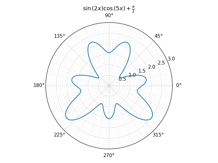
Polar plot with Matplotlib:

from sympy import symbols, sin, cos, pi, latex
from spb import plot_polar
x = symbols("x")
expr = sin(2 * x) * cos(5 * x) + pi / 2
plot_polar(expr, (x, 0, 2 * pi), ylim=(0, 3), title="$%s$" % latex(expr))

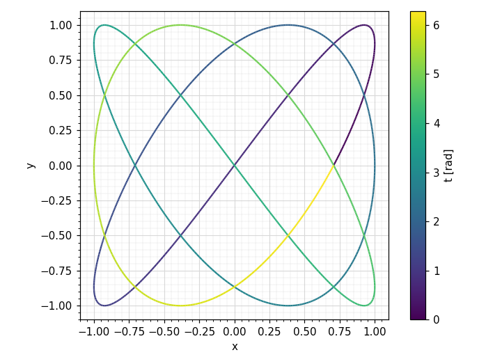
2D parametric plot with Matplotlib, using Numpy and lambda functions:

import numpy as np
from spb import plot_parametric
plot_parametric(
   lambda t: np.sin(3 * t + np.pi / 4), lambda t: np.sin(4 * t),
   ("t", 0, 2 * pi), "t [rad]", xlabel="x", ylabel="y", aspect="equal")

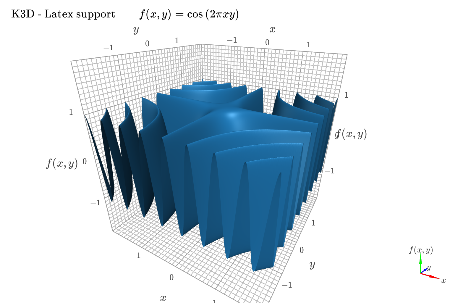
3D plot with K3D-Jupyter and cartesian discretization:

from sympy import symbols, cos, pi
from spb import plot3d, KB
x, y = symbols("x, y")
expr = cos(2 * pi * x * y)
title = r"\text{K3D - Latex Support} \qquad f(x, y) = " + latex(expr)
plot3d(
    expr, (x, -2, 2), (y, -2, 2),
    use_cm=False, n=300, title=title,
    backend=KB)

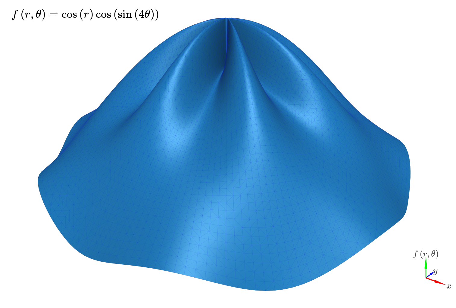
3D plot with K3D-Jupyter and polar discretization. Two identical expressions are going to be plotted, one will display the mesh with a solid color, the other will display the connectivity of the mesh (wireframe). Customization on the colors, surface/wireframe can easily be done after the plot is created:

from sympy import symbols, cos, sin, pi, latex
from spb import plot3d, KB
r, theta = symbols("r, theta")
expr = cos(r) * cos(sin(4 * theta))
plot3d(
    expr, expr, (r, 0, 2), (theta, 0, 2 * pi),
    n1=50, n2=200, is_polar=True, grid=False,
    title=r"f\left(r, \theta\right) = " + latex(expr), backend=KB)

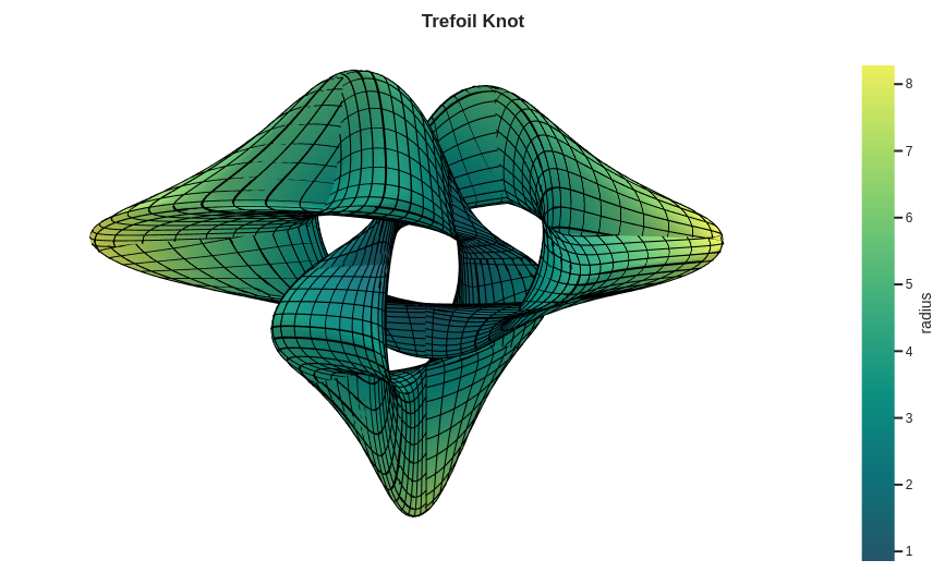
3D plot with Plotly of a parametric surface, colored according to the radius, with wireframe lines (also known as grid lines) highlighting the parameterization:

from sympy import symbols, cos, sin, pi
from spb import plot3d_parametric_surface, PB
import numpy as np
u, v = symbols("u, v")
def trefoil(u, v, r):
    x = r * sin(3 * u) / (2 + cos(v))
    y = r * (sin(u) + 2 * sin(2 * u)) / (2 + cos(v + pi * 2 / 3))
    z = r / 2 * (cos(u) - 2 * cos(2 * u)) * (2 + cos(v)) * (2 + cos(v + pi * 2 / 3)) / 4
    return x, y, z
plot3d_parametric_surface(
   trefoil(u, v, 3), (u, -pi, 3*pi), (v, -pi, 3*pi), "radius",
   grid=False, title="Trefoil Knot", backend=PB, use_cm=True,
   color_func=lambda x, y, z: np.sqrt(x**2 + y**2 + z**2),
   wireframe=True, wf_n1=100, wf_n2=30, n1=250)

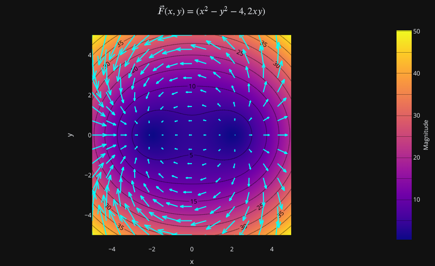
parametric surface plot with plotly showing wireframe lines

Visualizing a 2D vector field:

from sympy import symbols
from spb import plot_vector, PB
x, y = symbols("x, y")
expr = Tuple(x**2 - y**2 -4, 2 * x * y)
plot_vector(
    expr, (x, -5, 5), (y, -5, 5),
    backend=PB,
    n=15, quiver_kw={"scale":0.025},
    theme="plotly_dark",
    xlim=(-5, 5), ylim=(-5, 5),
    title=r"$\vec{F} = " + latex(expr) + "$")

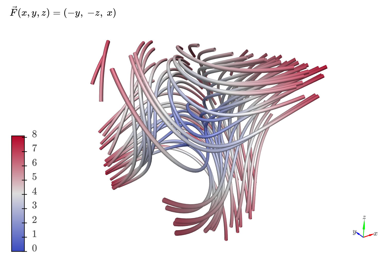
Visualizing a 3D vector field with a random number of streamtubes:

from sympy import symbols, Tuple
from spb import plot_vector, KB
x, y, z = symbols("x, y, z")
expr = Tuple(-y, -z, x)
plot_vector(
    expr, (x, -5, 5), (y, -5, 5), (z, -5, 5),
    streamlines=True, n=30,
    backend=KB, grid=False,
    stream_kw={"starts":True, "npoints":500},
    title=r"\vec{F}(x, y, z) = " + latex(expr))

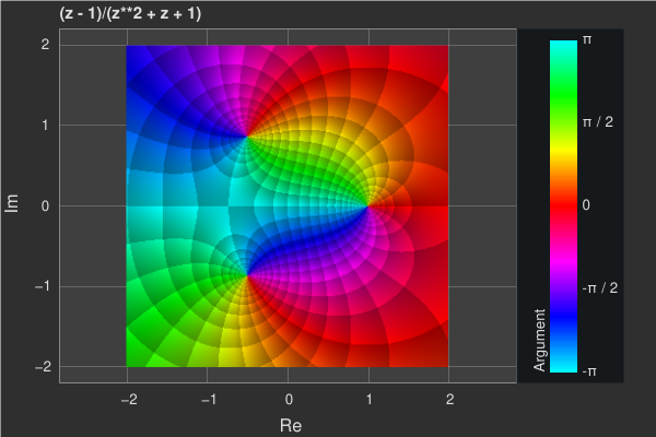
Domain coloring plot of a complex function:

from sympy import symbols
from spb import plot_complex, BB
z = symbols("z")
expr = (z - 1) / (z**2 + z + 1)
plot_complex(
    expr, (z, -2-2j, 2+2j),
    coloring="b",
    backend=BB, theme="dark_minimal",
    title=str(expr))

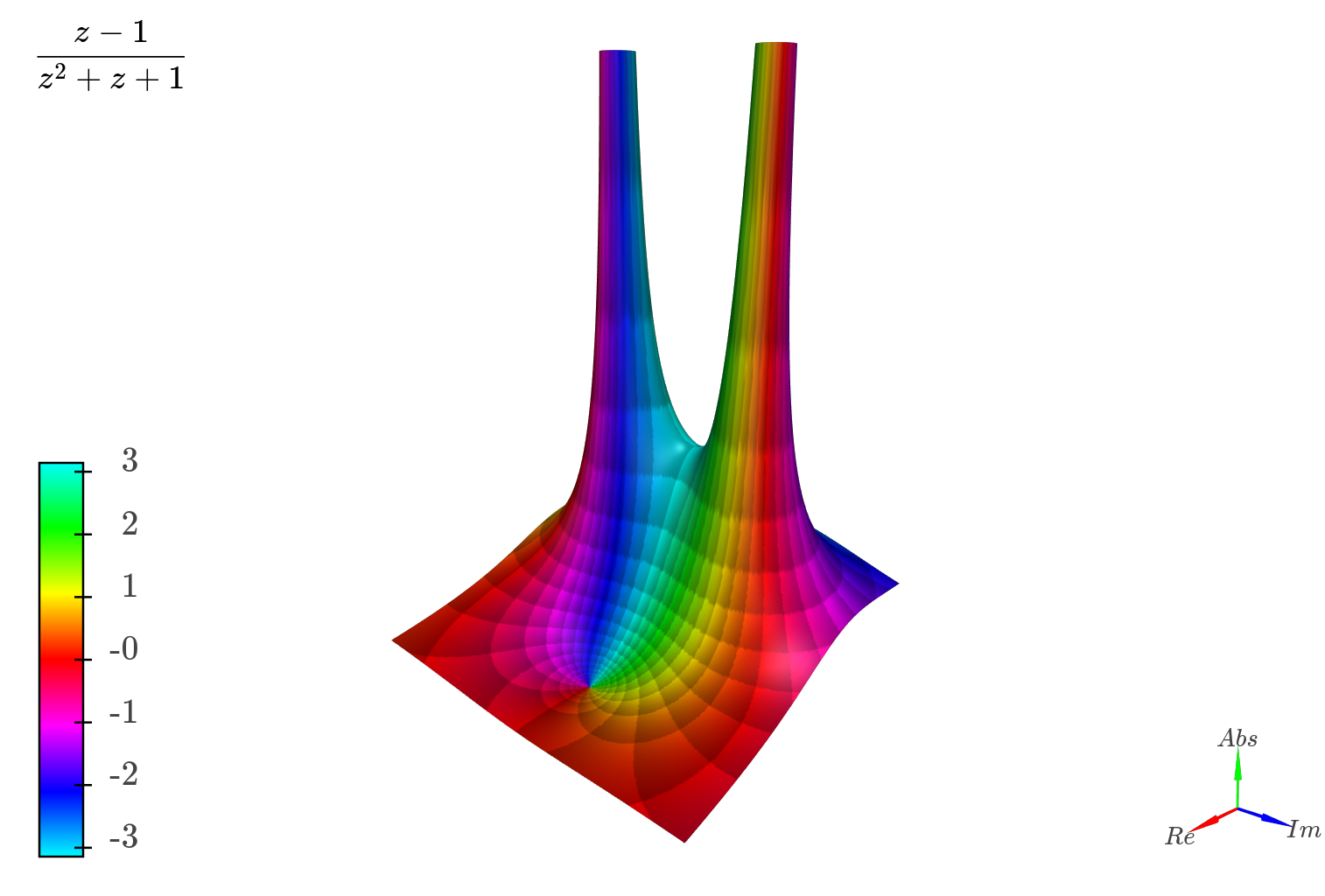
3D coloring plot of a complex function:

from sympy import symbols, latex
from spb import plot_complex, KB
z = symbols("z")
expr = (z - 1) / (z**2 + z + 1)
plot_complex(
    expr, (z, -2-2j, 2+2j),
    coloring="b", threed=True, zlim=(0, 6),
    backend=KB, grid=False,
    title=latex(expr))

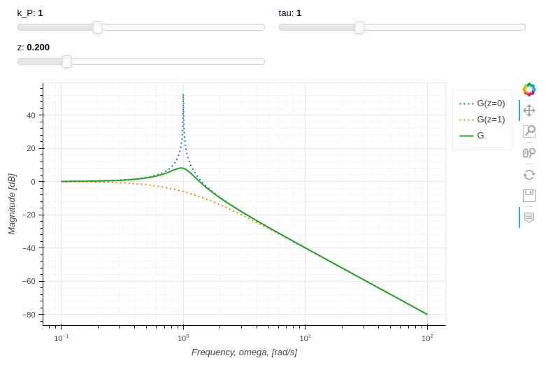
Interactive-Parametric 2D plot of the magnitude of a second order transfer function:

from sympy import symbols, log, sqrt, re, im, I
from spb import plot, BB
from bokeh.models.formatters import PrintfTickFormatter
formatter = PrintfTickFormatter(format="%.3f")
kp, t, z, o = symbols("k_P, tau, zeta, omega")
G = kp / (I**2 * t**2 * o**2 + 2 * z * t * o * I + 1)
mod = lambda x: 20 * log(sqrt(re(x)**2 + im(x)**2), 10)
plot(
    (mod(G.subs(z, 0)), (o, 0.1, 100), "G(z=0)", {"line_dash": "dotted"}),
    (mod(G.subs(z, 1)), (o, 0.1, 100), "G(z=1)", {"line_dash": "dotted"}),
    (mod(G), (o, 0.1, 100), "G"),
    params = {
        kp: (1, 0, 3),
        t: (1, 0, 3),
        z: (0.2, 0, 1, 200, formatter, "z")
    },
    backend = BB,
    n = 2000,
    xscale = "log",
    xlabel = "Frequency, omega, [rad/s]",
    ylabel = "Magnitude [dB]",
    use_latex = False
)

Differences with sympy.plotting

While the backends implemented in this module might resemble the ones from the sympy.plotting module, they are not interchangeable.
sympy.plotting also provides a Plotgrid class to combine multiple plots into a grid-like layout. This module replaces that class with the plotgrid function. Again, they are not interchangeable.
The plot_implicit function uses a mesh grid algorithm and contour plots by default (in contrast to the adaptive algorithm used by sympy.plotting). It is going to automatically switch to an adaptive algorithm if Boolean expressions are found. This ensures a better visualization for non-Boolean implicit expressions.
experimental_lambdify, used by sympy.plotting, has been completely removed.
sympy.plotting is unable to visualize summations containing infinity in their lower/upper bounds. The new module introduces the sum_bound keyword argument into the plot function: it substitutes infinity with a large integer number. As such, it is possible to visualize summations.
The adaptive algorithm is also different: this module relies on adaptive, which allows more flexibility.
- The depth keyword argument has been removed, while adaptive_goal and loss_fn have been introduced to control the new module.
- It has also been implemented to 3D lines and surfaces.
- It allows to generate smoother line plots, at the cost of performance.
sympy.plotting exposed the nb_of_points_* keyword arguments. These have been replaced with n or n1, n2.

sympy.plotting exposed the TextBackend class to create very basic plots on a terminal window. This module removed it.

The following example compares how to customize a plot created with sympy.plotting and one created with this module.

This is pretty much all we can do with sympy.plotting:

from sympy.plotting import plot
from sympy import symbols, sin, cos
x = symbols("x")
p = plot(sin(x), cos(x), show=False)
p[0].label = "a"
p[0].line_color = "red"
p[1].label = "b"
p.show()

The above command works perfectly fine also with this new module. However, we can customize the plot even further. In particular:

it is possible to set a custom label directly from any plot function.
the full potential of each backend can be accessed by providing dictionaries containing backend-specific keyword arguments.

from spb import plot
from sympy import symbols, sin, cos
x = symbols("x")
# pass customization options directly to matplotlib (or other backends)
plot(
    (sin(x), "a", dict(color="k", linestyle=":")),
    (cos(x), "b"),
    backend=MB)
# alternatively, set the label and rendering_kw keyword arguments
# to lists: each element target an expression
# plot(sin(x), cos(x), label=["a", "b"], rendering_kw=[dict(color="k", linestyle=":"), None])

Read the documentation to learn how to further customize the appearance of figures.

Take a look at Modules for more examples about the output of this module.