Complex

spb.ccomplex.complex.plot_complex(*args, **kwargs)[source]

Plot the absolute value of a complex function colored by its argument. By default, the aspect ratio of the plot is set to aspect="equal".

Depending on the provided range, this function will produce different types of plots:

Line plot over the reals.
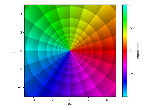
Image plot over the complex plane if threed=False. This is also known as Domain Coloring. Use the coloring keyword argument to select a different color scheme. At the moment, only HSV coloring is supported.
If threed=True, plot a 3D surface of the absolute value over the complex plane, colored by its argument. Use the coloring keyword argument to select a different color scheme. At the moment, only HSV coloring is supported.

Typical usage examples are in the followings:

Plotting a single expression with a single range.
plot_complex(expr, range, **kwargs)
Plotting a single expression with the default range (-10, 10).
plot_complex(expr, **kwargs)
Plotting multiple expressions with a single range.
plot_complex(expr1, expr2, …, range, **kwargs)
Plotting multiple expressions with multiple ranges.
plot_complex((expr1, range1), (expr2, range2), …, **kwargs)
Plotting multiple expressions with custom labels and rendering options.
plot_complex((expr1, range1, label1, rendering_kw1), (expr2, range2, label2, rendering_kw2), …, **kwargs)

Parameters

args

exprExpr or callable

Represent the complex function to be plotted. It can be a:

Symbolic expression.
Numerical function of one variable, supporting vectorization. In this case the following keyword arguments are not supported: params.

range3-element tuple

Denotes the range of the variables. For example:

(z, -5, 5): plot a line over the reals from point -5 to 5
(z, -5 + 2*I, 5 + 2*I): plot a line from complex point (-5 + 2*I) to (5 + 2 * I). Note the same imaginary part for the start/end point. Also note that we can specify the ranges by using standard Python complex numbers, for example (z, -5+2j, 5+2j).
(z, -5 - 3*I, 5 + 3*I): surface or contour plot of the complex function over the specified domain.

labelstr, optional

The name of the complex function to be eventually shown on the legend. If none is provided, the string representation of the function will be used.

rendering_kwdict, optional

A dictionary of keywords/values which is passed to the backend’s function to customize the appearance of lines, surfaces or images. Refer to the plotting library (backend) manual for more informations.

adaptivebool, optional

Attempt to create line plots by using an adaptive algorithm. Image and surface plots do not use an adaptive algorithm. Default to True. Use adaptive_goal and loss_fn to further customize the output.

adaptive_goalcallable, int, float or None

Controls the “smoothness” of the evaluation. Possible values:

None (default): it will use the following goal: lambda l: l.loss() < 0.01
number (int or float). The lower the number, the more evaluation points. This number will be used in the following goal: lambda l: l.loss() < number
callable: a function requiring one input element, the learner. It must return a float number. Refer to 2 for more information.

aspect(float, float) or str, optional

Set the aspect ratio of the plot. The value depends on the backend being used. Read that backend’s documentation to find out the possible values.

backendPlot, optional

A subclass of Plot, which will perform the rendering. Default to MatplotlibBackend.

labelstr or list/tuple, optional

The label to be shown in the legend or colorbar in case of a line plot. If not provided, the string representation of expr will be used. The number of labels must be equal to the number of expressions.

loss_fncallable or None

The loss function to be used by the adaptive learner. Possible values:

None (default): it will use the default_loss from the adaptive module.
callable : Refer to 2 for more information. Specifically, look at adaptive.learner.learner1D to find more loss functions.

modulesstr, optional

Specify the modules to be used for the numerical evaluation. Refer to lambdify to visualize the available options. Default to None, meaning Numpy/Scipy will be used. Note that other modules might produce different results, based on the way they deal with branch cuts.

n1, n2int, optional

Number of discretization points in the real/imaginary-directions, respectively, when adaptive=False. For line plots, default to 1000. For surface/contour plots (2D and 3D), default to 300.

nint or two-elements tuple (n1, n2), optional

If an integer is provided, set the same number of discretization points in all directions. If a tuple is provided, it overrides n1 and n2. It only works when adaptive=False.

paramsdict

A dictionary mapping symbols to parameters. This keyword argument enables the interactive-widgets plot, which doesn’t support the adaptive algorithm (meaning it will use adaptive=False). Learn more by reading the documentation of iplot.

rendering_kwdict or list of dicts, optional

A dictionary of keywords/values which is passed to the backend’s function to customize the appearance of lines, surfaces or images. Refer to the plotting library (backend) manual for more informations. If a list of dictionaries is provided, the number of dictionaries must be equal to the number of series generated by the plotting function.

showboolean, optional

Default to True, in which case the plot will be shown on the screen.

size(float, float), optional

A tuple in the form (width, height) to specify the size of the overall figure. The default value is set to None, meaning the size will be set by the backend.

threedboolean, optional

It only applies to a complex function over a complex range. If False, a 2D image plot will be shown. If True, 3D surfaces will be shown. Default to False.

coloringstr or callable

Choose between different domain coloring options. Default to “a”. Refer to 1 for more information.

“a”: standard domain coloring using HSV, showing the argument of the complex function.
“b”: enhanced domain coloring using HSV, showing iso-modulus and is-phase lines.
“c”: enhanced domain coloring using HSV, showing iso-modulus lines.
“d”: enhanced domain coloring using HSV, showing iso-phase lines.
“e”: alternating black and white stripes corresponding to modulus.
“f”: alternating black and white stripes corresponding to phase.
“g”: alternating black and white stripes corresponding to real part.
“h”: alternating black and white stripes corresponding to imaginary part.
“i”: cartesian chessboard on the complex points space. The result will hide zeros.
“j”: polar Chessboard on the complex points space. The result will show conformality.

The user can also provide a callable, f(w), where w is an [n x m] Numpy array (provided by the plotting module) containing the results (complex numbers) of the evaluation of the complex function. The callable should return:

imgndarray [n x m x 3]
An array of RGB colors (0 <= R,G,B <= 255)
colorscalendarray [N x 3] or None
An array with N RGB colors, (0 <= R,G,B <= 255). If colorscale=None, no color bar will be shown on the plot.

phaseresint

Default value to 20. It controls the number of iso-phase and/or iso-modulus lines in domain coloring plots.

titlestr, optional

Title of the plot. It is set to the latex representation of the expression, if the plot has only one expression.

use_latexboolean, optional

Turn on/off the rendering of latex labels. If the backend doesn’t support latex, it will render the string representations instead.

xlabelstr, optional

Label for the x-axis.

ylabelstr, optional

Label for the y-axis.

zlabelstr, optional

Label for the z-axis. Only available for 3D plots.

xscale‘linear’ or ‘log’, optional

Sets the scaling of the x-axis. Default to ‘linear’.

yscale‘linear’ or ‘log’, optional

Sets the scaling of the y-axis. Default to ‘linear’.

xlim(float, float), optional

Denotes the x-axis limits, (min, max).

ylim(float, float), optional

Denotes the y-axis limits, (min, max).

zlim(float, float), optional

Denotes the z-axis limits, (min, max). Only available for 3D plots.

See also

plot_real_imag, plot_complex_list, plot_complex_vector, iplot

References

1: Domain Coloring is based on Elias Wegert’s book “Visual Complex Functions”. The book provides the background to better understand the images.
2(1,2): https://github.com/python-adaptive/adaptive

Examples

>>> from sympy import I, symbols, exp, sqrt, cos, sin, pi, gamma
>>> from spb import plot_complex
>>> x, y, z = symbols('x, y, z')

(Source code)

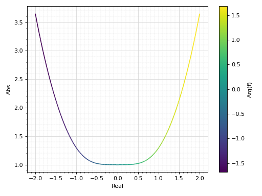
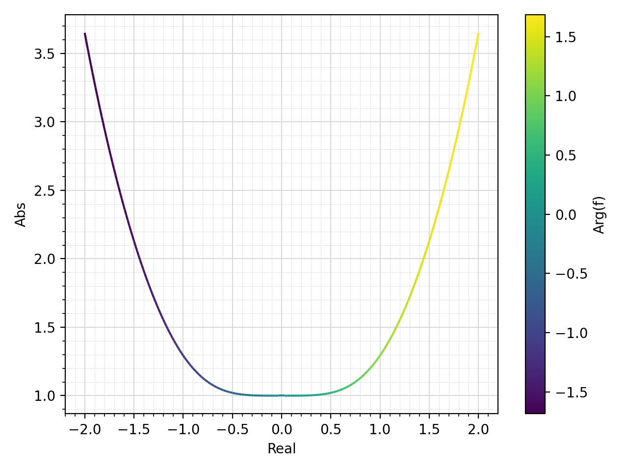
Plot the modulus of a complex function colored by its magnitude:

>>> plot_complex(cos(x) + sin(I * x), "f", (x, -2, 2))
Plot object containing:
[0]: cartesian abs-arg line: cos(x) + I*sinh(x) for x over ((-2+0j), (2+0j))

(Source code, png, hires.png, pdf)

Interactive-widget plot. Refer to iplot documentation to learn more about the params dictionary.

from sympy import *
x, u = symbols("x, u")
plot_complex(
    exp(I * x) * I * sin(u * x), "f", (x, -5, 5),
    params={u: (1, 0, 2)}, ylim=(-0.2, 1.2))

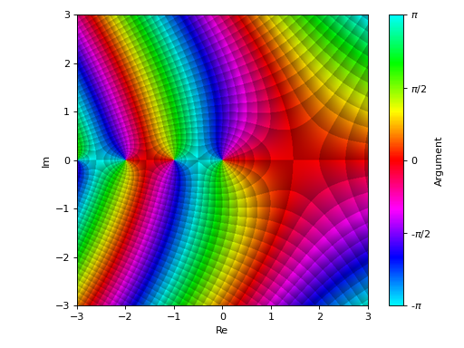
Domain coloring plot. To improve the smoothness of the results, increase the number of discretization points and/or apply an interpolation (if the backend supports it):

>>> plot_complex(gamma(z), (z, -3-3j, 3+3j),
...     {"interpolation": "spline36"}, # passed to matplotlib's imshow
...     coloring="b", n=500, grid=False)
Plot object containing:
[0]: complex domain coloring: gamma(z) for re(z) over (-3.0, 3.0) and im(z) over (-3.0, 3.0)

(Source code, png, hires.png, pdf)

Plotting a numerical function instead of a symbolic expression:

>>> import numpy as np
>>> plot_complex(lambda z: z, ("z", -5-5j, 5+5j),
...     {"interpolation": "spline36"}, # passed to matplotlib's imshow
...     coloring="b", n=600, grid=False)

(Source code, png, hires.png, pdf)

Interactive-widget domain coloring plot. Refer to iplot documentation to learn more about the params dictionary. Note that a too large value of n will impact performance.

from sympy import *
x, u = symbols("x, u")
plot_complex(
    gamma(u * z), (z, -3 - 3*I, 3 + 3*I),
    coloring="b", n=250, grid=False, params={u: (1, 0, 2)})

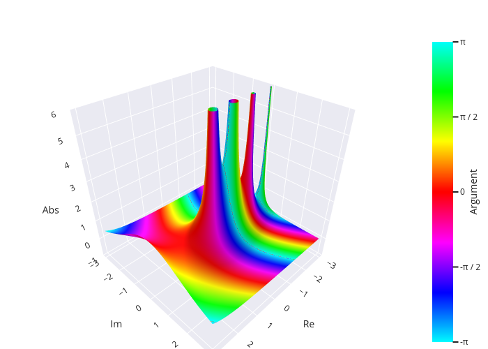
3D plot of the absolute value of a complex function colored by its argument, using Plotly:

from sympy import symbols, gamma, I
from spb import plot_complex, PB
z = symbols('z')
plot_complex(gamma(z), (z, -3 - 3*I, 3 + 3*I), threed=True,
    backend=PB, zlim=(-1, 6), use_cm=True)

(Source code, png, html, pdf)

spb.ccomplex.complex.plot_complex_list(*args, **kwargs)[source]

Plot lists of complex points. By default, the aspect ratio of the plot is set to aspect="equal".

Typical usage examples are in the followings:

Plotting a single list of complex numbers.
plot_complex_list(l1, **kwargs)
Plotting multiple lists of complex numbers.
plot_complex_list(l1, l2, **kwargs)
Plotting multiple lists of complex numbers each one with a custom label.
plot_complex_list((l1, label1), (l2, label2), **kwargs)

Parameters

args

numberslist, tuple: A list of complex numbers.
labelstr: The name associated to the list of the complex numbers to be eventually shown on the legend. Default to empty string.
rendering_kwdict, optional: A dictionary of keywords/values which is passed to the backend’s function to customize the appearance of lines. Refer to the plotting library (backend) manual for more informations. Note that the same options will be applied to all series generated for the specified expression.

aspect(float, float) or str, optional

Set the aspect ratio of the plot. The value depends on the backend being used. Read that backend’s documentation to find out the possible values.

backendPlot, optional

A subclass of Plot, which will perform the rendering. Default to MatplotlibBackend.

is_pointboolean

If True, a scatter plot will be produced. Otherwise a line plot will be created. Default to True.

is_filledboolean, optional

Default to True, which will render empty circular markers. It only works if is_point=True. If False, filled circular markers will be rendered.

labelstr or list/tuple, optional

The name associated to the list of the complex numbers to be eventually shown on the legend. The number of labels must be equal to the number of series generated by the plotting function.

paramsdict

A dictionary mapping symbols to parameters. This keyword argument enables the interactive-widgets plot, which doesn’t support the adaptive algorithm (meaning it will use adaptive=False). Learn more by reading the documentation of iplot.

rendering_kwdict or list of dicts, optional

A dictionary of keywords/values which is passed to the backend’s function to customize the appearance of lines. Refer to the plotting library (backend) manual for more informations. If a list of dictionaries is provided, the number of dictionaries must be equal to the number of series generated by the plotting function.

showboolean

Default to True, in which case the plot will be shown on the screen.

size(float, float), optional

A tuple in the form (width, height) to specify the size of the overall figure. The default value is set to None, meaning the size will be set by the backend.

titlestr, optional

Title of the plot. It is set to the latex representation of the expression, if the plot has only one expression.

use_latexboolean, optional

Turn on/off the rendering of latex labels. If the backend doesn’t support latex, it will render the string representations instead.

xlabelstr, optional

Label for the x-axis.

ylabelstr, optional

Label for the y-axis.

xscale‘linear’ or ‘log’, optional

Sets the scaling of the x-axis. Default to ‘linear’.

yscale‘linear’ or ‘log’, optional

Sets the scaling of the y-axis. Default to ‘linear’.

xlim(float, float), optional

Denotes the x-axis limits, (min, max).

ylim(float, float), optional

Denotes the y-axis limits, (min, max).

See also

plot_real_imag, plot_complex, plot_complex_vector, iplot

Examples

>>> from sympy import I, symbols, exp, sqrt, cos, sin, pi, gamma
>>> from spb import plot_complex_list
>>> x, y, z = symbols('x, y, z')

(Source code)

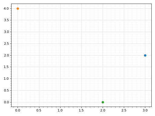
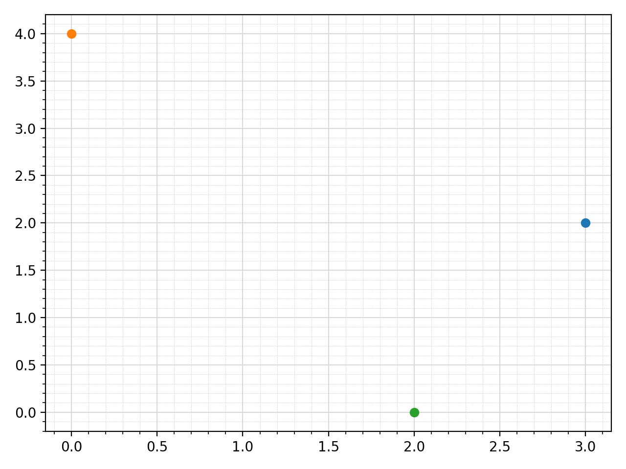
Plot individual complex points:

>>> plot_complex_list(3 + 2 * I, 4 * I, 2)
Plot object containing:
[0]: complex points: (3 + 2*I,)
[1]: complex points: (4*I,)
[2]: complex points: (2,)

(Source code, png, hires.png, pdf)

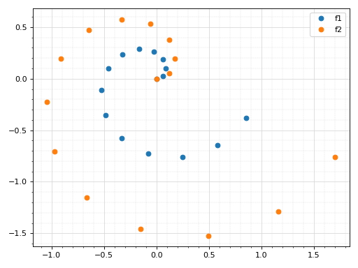
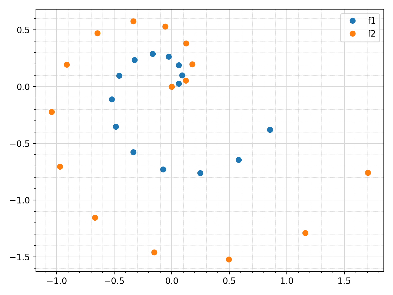
Plot two lists of complex points and assign to them custom labels:

>>> expr1 = z * exp(2 * pi * I * z)
>>> expr2 = 2 * expr1
>>> n = 15
>>> l1 = [expr1.subs(z, t / n) for t in range(n)]
>>> l2 = [expr2.subs(z, t / n) for t in range(n)]
>>> plot_complex_list((l1, "f1"), (l2, "f2"))
Plot object containing:
[0]: complex points: (0.0, 0.0666666666666667*exp(0.133333333333333*I*pi), 0.133333333333333*exp(0.266666666666667*I*pi), 0.2*exp(0.4*I*pi), 0.266666666666667*exp(0.533333333333333*I*pi), 0.333333333333333*exp(0.666666666666667*I*pi), 0.4*exp(0.8*I*pi), 0.466666666666667*exp(0.933333333333333*I*pi), 0.533333333333333*exp(1.06666666666667*I*pi), 0.6*exp(1.2*I*pi), 0.666666666666667*exp(1.33333333333333*I*pi), 0.733333333333333*exp(1.46666666666667*I*pi), 0.8*exp(1.6*I*pi), 0.866666666666667*exp(1.73333333333333*I*pi), 0.933333333333333*exp(1.86666666666667*I*pi))
[1]: complex points: (0, 0.133333333333333*exp(0.133333333333333*I*pi), 0.266666666666667*exp(0.266666666666667*I*pi), 0.4*exp(0.4*I*pi), 0.533333333333333*exp(0.533333333333333*I*pi), 0.666666666666667*exp(0.666666666666667*I*pi), 0.8*exp(0.8*I*pi), 0.933333333333333*exp(0.933333333333333*I*pi), 1.06666666666667*exp(1.06666666666667*I*pi), 1.2*exp(1.2*I*pi), 1.33333333333333*exp(1.33333333333333*I*pi), 1.46666666666667*exp(1.46666666666667*I*pi), 1.6*exp(1.6*I*pi), 1.73333333333333*exp(1.73333333333333*I*pi), 1.86666666666667*exp(1.86666666666667*I*pi))

(Source code, png, hires.png, pdf)

Interactive-widget plot. Refer to iplot documentation to learn more about the params dictionary.

from sympy import *
z, u = symbols("z u")
expr1 = z * exp(2 * pi * I * z)
expr2 = u * expr1
n = 15
l1 = [expr1.subs(z, t / n) for t in range(n)]
l2 = [expr2.subs(z, t / n) for t in range(n)]
plot_complex_list(
    (l1, "f1"), (l2, "f2"),
    params={u: (0.5, 0, 2)},
    xlim=(-1.5, 2), ylim=(-2, 1))

spb.ccomplex.complex.plot_real_imag(*args, **kwargs)[source]

Plot the real part, the imaginary parts, the absolute value and the argument of a complex function. By default, only the real and imaginary parts will be plotted. Use keyword argument to be more specific. By default, the aspect ratio of the plot is set to aspect="equal".

Depending on the provided expression, this function will produce different types of plots:

line plot over the reals.
surface plot over the complex plane if threed=True.
contour plot over the complex plane if threed=False.

Typical usage examples are in the followings:

Plotting a single expression with a single range.
plot_real_imag(expr, range, **kwargs)
Plotting a single expression with the default range (-10, 10).
plot_real_imag(expr, **kwargs)
Plotting multiple expressions with a single range.
plot_real_imag(expr1, expr2, …, range, **kwargs)
Plotting multiple expressions with multiple ranges.
plot_real_imag((expr1, range1), (expr2, range2), …, **kwargs)
Plotting multiple expressions with custom labels and rendering options.
plot_real_imag((expr1, range1, label1, rendering_kw1), (expr2, range2, label2, rendering_kw2), …, **kwargs)

Parameters

args

exprExpr

Represent the complex function to be plotted.

range3-element tuple

Denotes the range of the variables. For example:

(z, -5, 5): plot a line over the reals from point -5 to 5
(z, -5 + 2*I, 5 + 2*I): plot a line from complex point (-5 + 2*I) to (5 + 2 * I). Note the same imaginary part for the start/end point. Also note that we can specify the ranges by using standard Python complex numbers, for example (z, -5+2j, 5+2j).
(z, -5 - 3*I, 5 + 3*I): surface or contour plot of the complex function over the specified domain using a rectangular discretization.

labelstr, optional

The name of the complex function to be eventually shown on the legend. If none is provided, the string representation of the function will be used.

rendering_kwdict, optional

A dictionary of keywords/values which is passed to the backend’s function to customize the appearance of lines. Refer to the plotting library (backend) manual for more informations. Note that the same options will be applied to all series generated for the specified expression.

absboolean, optional

If True, plot the modulus of the complex function. Default to True.

adaptivebool, optional

Attempt to create line plots by using an adaptive algorithm. Image and surface plots do not use an adaptive algorithm. Default to True. Use adaptive_goal and loss_fn to further customize the output.

adaptive_goalcallable, int, float or None

Controls the “smoothness” of the evaluation. Possible values:

None (default): it will use the following goal: lambda l: l.loss() < 0.01
number (int or float). The lower the number, the more evaluation points. This number will be used in the following goal: lambda l: l.loss() < number
callable: a function requiring one input element, the learner. It must return a float number. Refer to 3 for more information.

argboolean, optional

If True, plot the argument of the complex function. Default to True.

aspect(float, float) or str, optional

Set the aspect ratio of the plot. The value depends on the backend being used. Read that backend’s documentation to find out the possible values.

backendPlot, optional

A subclass of Plot, which will perform the rendering. Default to MatplotlibBackend.

detect_polesboolean, optional

Chose whether to detect and correctly plot poles. Defaulto to False. It only works with line plots. To improve detection, increase the number of discretization points if adaptive=False and/or change the value of eps.

epsfloat, optional

An arbitrary small value used by the detect_poles algorithm. Default value to 0.1. Before changing this value, it is better to increase the number of discretization points.

imagboolean, optional

If True, plot the imaginary part of the complex function. Default to True.

labellist/tuple, optional

The labels to be shown in the legend. If not provided, the string representation of expr will be used. The number of labels must be equal to the number of series generated by the plotting function.

loss_fncallable or None

The loss function to be used by the adaptive learner. Possible values:

None (default): it will use the default_loss from the adaptive module.
callable : Refer to 3 for more information. Specifically, look at adaptive.learner.learner1D to find more loss functions.

modulesstr, optional

Specify the modules to be used for the numerical evaluation. Refer to lambdify to visualize the available options. Default to None, meaning Numpy/Scipy will be used. Note that other modules might produce different results, based on the way they deal with branch cuts.

n1, n2int, optional

Number of discretization points in the real/imaginary-directions, respectively, when adaptive=False. For line plots, default to 1000. For surface/contour plots (2D and 3D), default to 300.

nint or two-elements tuple (n1, n2), optional

If an integer is provided, set the same number of discretization points in all directions. If a tuple is provided, it overrides n1 and n2. It only works when adaptive=False.

paramsdict

A dictionary mapping symbols to parameters. This keyword argument enables the interactive-widgets plot, which doesn’t support the adaptive algorithm (meaning it will use adaptive=False). Learn more by reading the documentation of iplot.

rendering_kwdict or list of dicts, optional

A dictionary of keywords/values which is passed to the backend’s function to customize the appearance of lines. Refer to the plotting library (backend) manual for more informations. If a list of dictionaries is provided, the number of dictionaries must be equal to the number of series generated by the plotting function.

realboolean, optional

If True, plot the real part of the complex function. Default to True.

showboolean, optional

Default to True, in which case the plot will be shown on the screen.

size(float, float), optional

A tuple in the form (width, height) to specify the size of the overall figure. The default value is set to None, meaning the size will be set by the backend.

surface_kwdict, optional

A dictionary of keywords/values which is passed to the backend’s function to customize the appearance of surfaces. Refer to the plotting library (backend) manual for more informations.

threedboolean, optional

It only applies to a complex function over a complex range. If False, contour plots will be shown. If True, 3D surfaces will be shown. Default to False.

use_cmboolean, optional

If False, surfaces will be rendered with a solid color. If True, a color map highlighting the elevation will be used. Default to True.

use_latexboolean, optional

Turn on/off the rendering of latex labels. If the backend doesn’t support latex, it will render the string representations instead.

titlestr, optional

Title of the plot. It is set to the latex representation of the expression, if the plot has only one expression.

xlabelstr, optional

Label for the x-axis.

ylabelstr, optional

Label for the y-axis.

zlabelstr, optional

Label for the z-axis. Only available for 3D plots.

xscale‘linear’ or ‘log’, optional

Sets the scaling of the x-axis. Default to ‘linear’.

yscale‘linear’ or ‘log’, optional

Sets the scaling of the y-axis. Default to ‘linear’.

xlim(float, float), optional

Denotes the x-axis limits, (min, max).

ylim(float, float), optional

Denotes the y-axis limits, (min, max).

zlim(float, float), optional

Denotes the z-axis limits, (min, max). Only available for 3D plots.

See also

plot_complex, plot_complex_list, plot_complex_vector, iplot

References

3(1,2): https://github.com/python-adaptive/adaptive

Examples

>>> from sympy import I, symbols, exp, sqrt, cos, sin, pi, gamma
>>> from spb import plot_real_imag
>>> x, y, z = symbols('x, y, z')

(Source code)

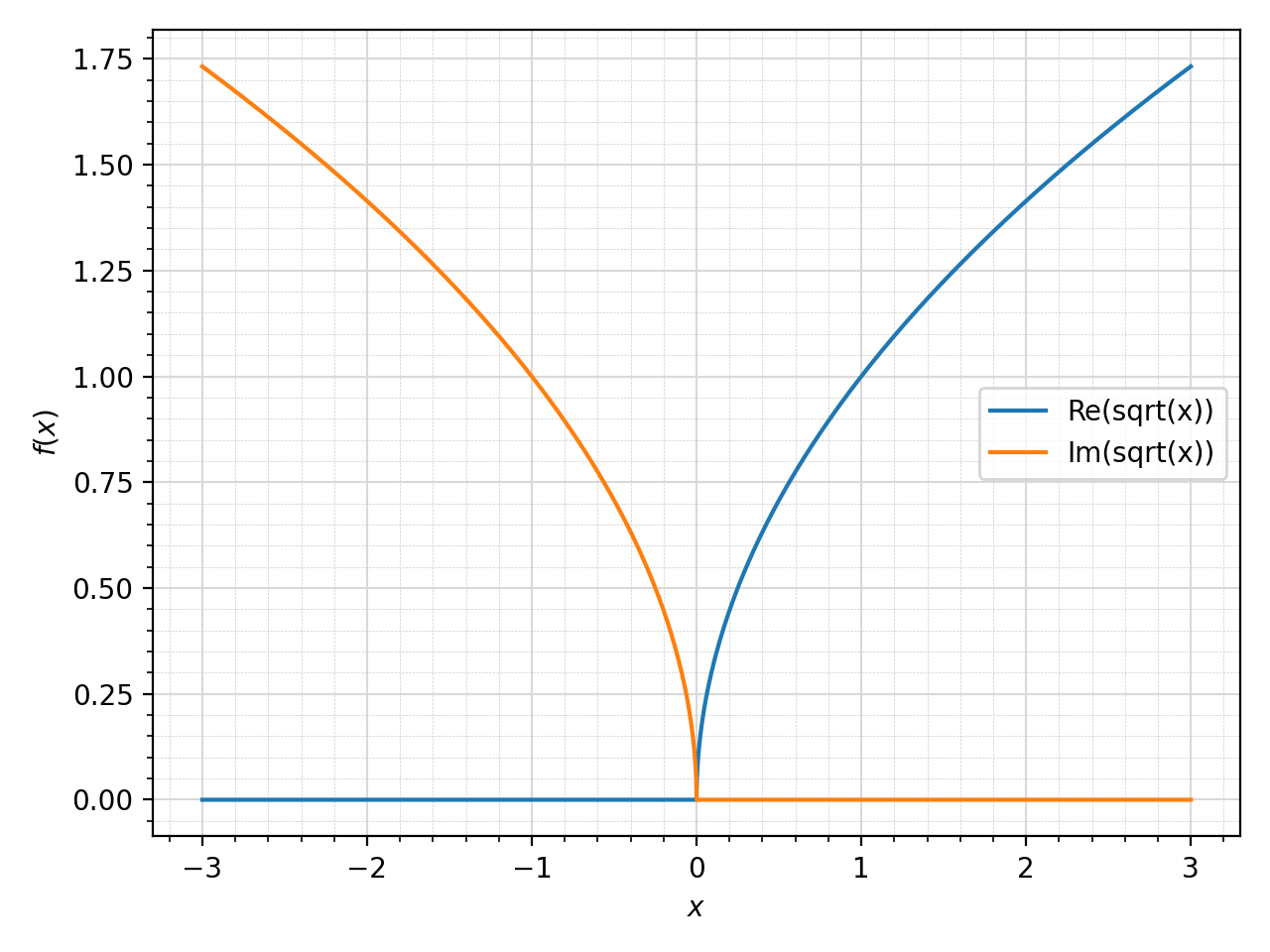
Plot the real and imaginary parts of a function over reals:

>>> plot_real_imag(sqrt(x), (x, -3, 3))
Plot object containing:
[0]: cartesian line: (re(x)**2 + im(x)**2)**(1/4)*cos(atan2(im(x), re(x))/2) for x over (-3.0, 3.0)
[1]: cartesian line: (re(x)**2 + im(x)**2)**(1/4)*sin(atan2(im(x), re(x))/2) for x over (-3.0, 3.0)

(Source code, png, hires.png, pdf)

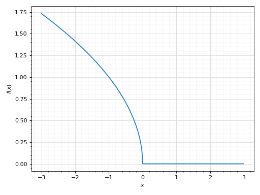
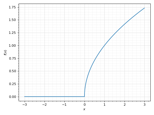
Plot only the real part:

>>> plot_real_imag(sqrt(x), (x, -3, 3), imag=False)
Plot object containing:
[0]: cartesian line: (re(x)**2 + im(x)**2)**(1/4)*cos(atan2(im(x), re(x))/2) for x over (-3.0, 3.0)

(Source code, png, hires.png, pdf)

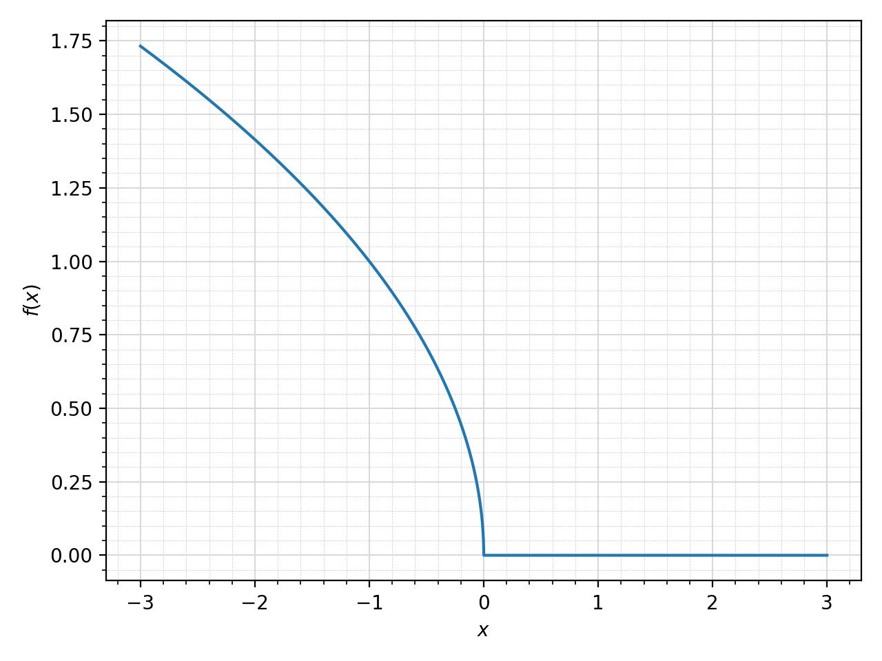
Plot only the imaginary part:

>>> plot_real_imag(sqrt(x), (x, -3, 3), real=False)
Plot object containing:
[0]: cartesian line: (re(x)**2 + im(x)**2)**(1/4)*sin(atan2(im(x), re(x))/2) for x over (-3.0, 3.0)

(Source code, png, hires.png, pdf)

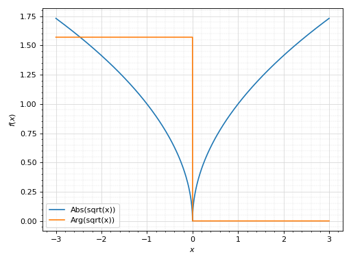
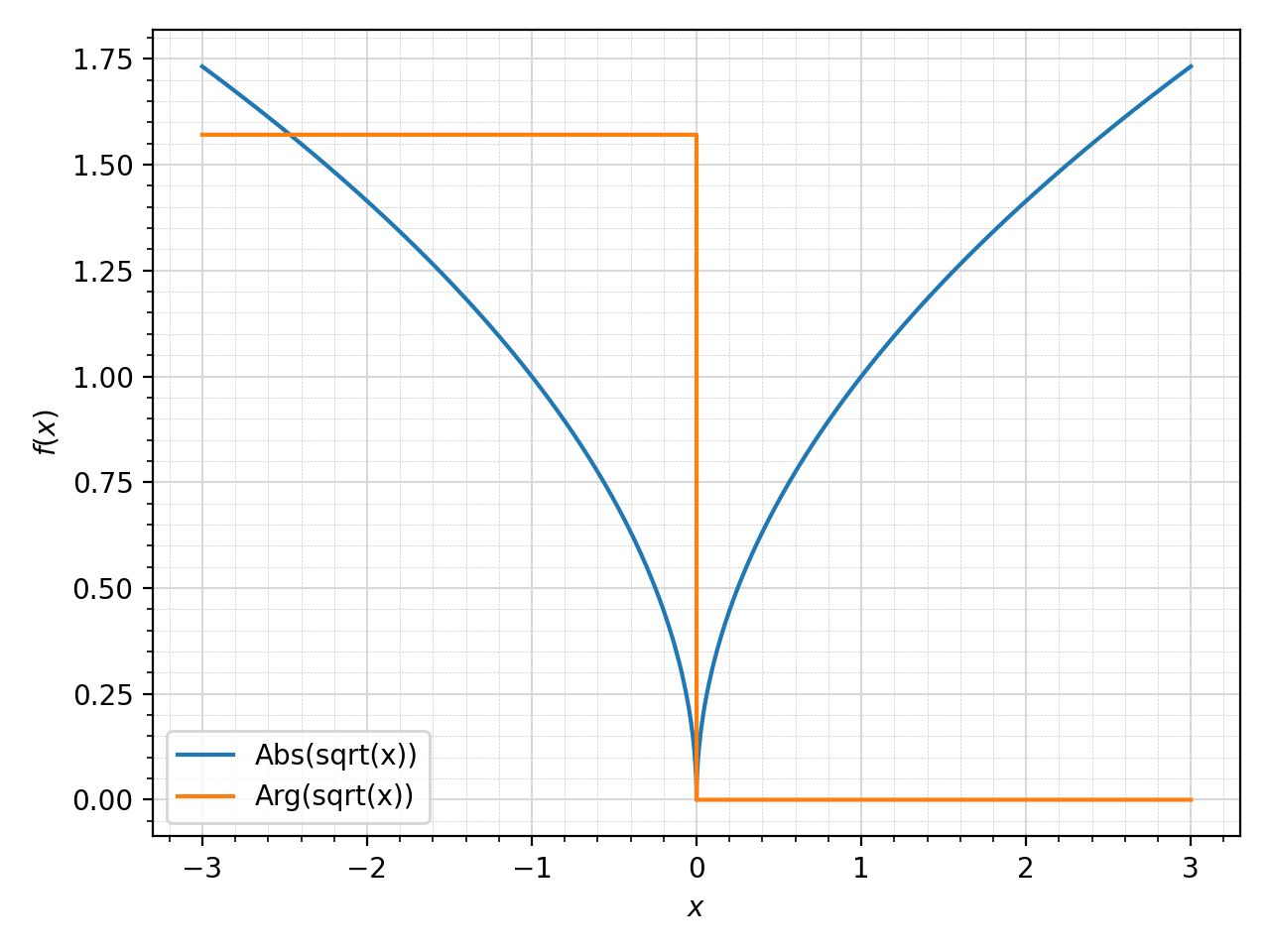
Plot only the absolute value and argument:

>>> plot_real_imag(sqrt(x), (x, -3, 3), real=False, imag=False, abs=True, arg=True)
Plot object containing:
[0]: cartesian line: sqrt(sqrt(re(x)**2 + im(x)**2)*sin(atan2(im(x), re(x))/2)**2 + sqrt(re(x)**2 + im(x)**2)*cos(atan2(im(x), re(x))/2)**2) for x over (-3.0, 3.0)
[1]: cartesian line: arg(sqrt(x)) for x over (-3.0, 3.0)

(Source code, png, hires.png, pdf)

Interactive-widget plot. Refer to iplot documentation to learn more about the params dictionary.

from sympy import *
x, u = symbols("x, u")
plot_real_imag(sqrt(x) * exp(-u * x**2), (x, -3, 3),
    params={u: (1, 0, 2)}, ylim=(-0.25, 2))

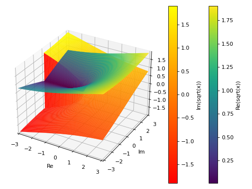
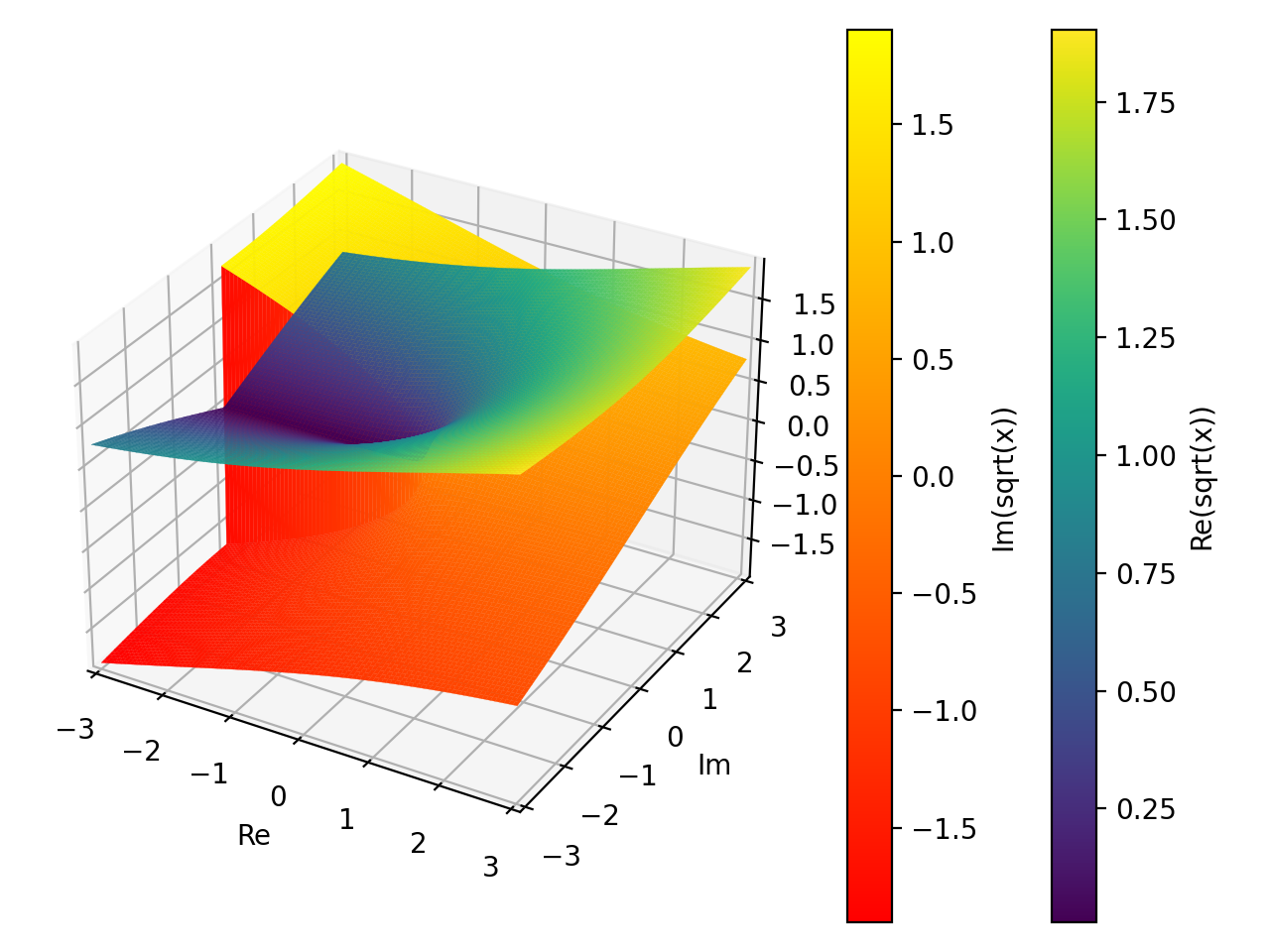
3D plot of the real and imaginary part of the principal branch of a function over a complex range. Note the jump in the imaginary part: that’s a branch cut. The rectangular discretization is unable to properly capture it, hence the near vertical wall. Refer to plot3d_parametric_surface for an example about plotting Riemann surfaces and properly capture the branch cuts.

>>> plot_real_imag(sqrt(x), (x, -3-3j, 3+3j), n=100, threed=True,
...      use_cm=True)
Plot object containing:
[0]: complex cartesian surface: (re(x)**2 + im(x)**2)**(1/4)*cos(atan2(im(x), re(x))/2) for re(x) over (-3.0, 3.0) and im(x) over (-3.0, 3.0)
[1]: complex cartesian surface: (re(x)**2 + im(x)**2)**(1/4)*sin(atan2(im(x), re(x))/2) for re(x) over (-3.0, 3.0) and im(x) over (-3.0, 3.0)

(Source code, png, hires.png, pdf)

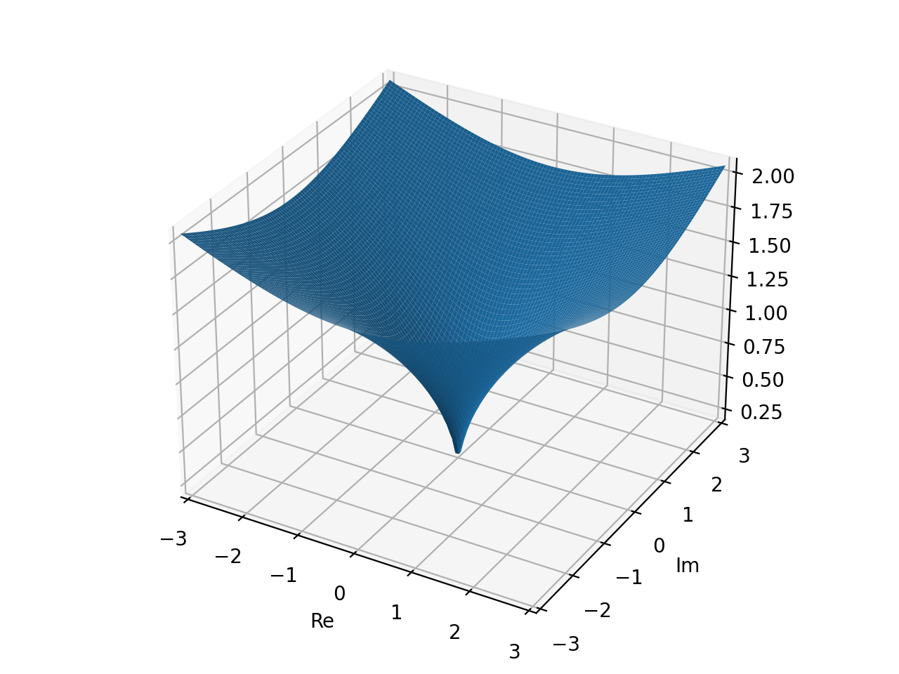
3D plot of the absolute value of a function over a complex range:

>>> plot_real_imag(sqrt(x), (x, -3-3j, 3+3j),
...     n=100, real=False, imag=False, abs=True, threed=True)
Plot object containing:
[0]: complex cartesian surface: sqrt(sqrt(re(x)**2 + im(x)**2)*sin(atan2(im(x), re(x))/2)**2 + sqrt(re(x)**2 + im(x)**2)*cos(atan2(im(x), re(x))/2)**2) for re(x) over (-3.0, 3.0) and im(x) over (-3.0, 3.0)

(Source code, png, hires.png, pdf)

3D interactive-widget plot. Refer to iplot documentation to learn more about the params dictionary.

from sympy import *
x, u = symbols("x, u")
plot_real_imag(
    sqrt(x) * exp(u * x), (x, -3-3j, 3+3j),
    params={u: (0.5, 0, 1)}, n=25, threed=True)

spb.ccomplex.complex.plot_complex_vector(*args, **kwargs)[source]

Plot the vector field [re(f), im(f)] for a complex function f over the specified complex domain. By default, the aspect ratio of the plot is set to aspect="equal".

Typical usage examples are in the followings:

Plotting a vector field of a complex function.
plot_complex_vector(expr, range, **kwargs)
Plotting multiple vector fields with different ranges and custom labels.
plot_complex_vector((expr1, range1, label1 [optional]), (expr2, range2, label2 [optional]), **kwargs)

Parameters

args

exprExpr: Represent the complex function.
range3-element tuples: Denotes the range of the variables. For example (z, -5 - 3*I, 5 + 3*I). Note that we can specify the range by using standard Python complex numbers, for example (z, -5-3j, 5+3j).
labelstr, optional: The name of the complex expression to be eventually shown on the legend. If none is provided, the string representation of the expression will be used.

aspect(float, float) or str, optional

Set the aspect ratio of the plot. The value depends on the backend being used. Read that backend’s documentation to find out the possible values.

backendPlot, optional

A subclass of Plot, which will perform the rendering. Default to MatplotlibBackend.

contours_kwdict

A dictionary of keywords/values which is passed to the backend contour function to customize the appearance. Refer to the plotting library (backend) manual for more informations.

n1, n2int

Number of discretization points for the quivers or streamlines in the x/y-direction, respectively. Default to 25.

nint or two-elements tuple (n1, n2), optional

If an integer is provided, set the same number of discretization points in all directions for quivers or streamlines. If a tuple is provided, it overrides n1 and n2. It only works when adaptive=False. Default to 25.

ncint

Number of discretization points for the scalar contour plot. Default to 100.

paramsdict

A dictionary mapping symbols to parameters. This keyword argument enables the interactive-widgets plot, which doesn’t support the adaptive algorithm (meaning it will use adaptive=False). Learn more by reading the documentation of iplot.

quiver_kwdict

A dictionary of keywords/values which is passed to the backend quivers-plotting function to customize the appearance. Refer to the plotting library (backend) manual for more informations.

scalarboolean, Expr, None or list/tuple of 2 elements

Represents the scalar field to be plotted in the background of a 2D vector field plot. Can be:

True: plot the magnitude of the vector field. Only works when a single vector field is plotted.
False/None: do not plot any scalar field.
Expr: a symbolic expression representing the scalar field.
list/tuple: [scalar_expr, label], where the label will be shown on the colorbar.

Remember: the scalar function must return real data.

Default to True.

showboolean

The default value is set to True. Set show to False and the function will not display the plot. The returned instance of the Plot class can then be used to save or display the plot by calling the save() and show() methods respectively.

size(float, float), optional

A tuple in the form (width, height) to specify the size of the overall figure. The default value is set to None, meaning the size will be set by the backend.

streamlinesboolean

Whether to plot the vector field using streamlines (True) or quivers (False). Default to False.

stream_kwdict

A dictionary of keywords/values which is passed to the backend streamlines-plotting function to customize the appearance. Refer to the plotting library (backend) manual for more informations.

titlestr, optional

Title of the plot. It is set to the latex representation of the expression, if the plot has only one expression.

use_latexboolean, optional

Turn on/off the rendering of latex labels. If the backend doesn’t support latex, it will render the string representations instead.

xlabelstr, optional

Label for the x-axis.

ylabelstr, optional

Label for the y-axis.

xscale‘linear’ or ‘log’, optional

Sets the scaling of the x-axis. Default to ‘linear’.

yscale‘linear’ or ‘log’, optional

Sets the scaling of the y-axis. Default to ‘linear’.

xlim(float, float), optional

Denotes the x-axis limits, (min, max).

ylim(float, float), optional

Denotes the y-axis limits, (min, max).

See also

plot_real_imag, plot_complex, plot_complex_list, plot_vector, iplot

Examples

>>> from sympy import I, symbols, gamma, latex, log
>>> from spb import plot_complex_vector, plot_complex
>>> z = symbols('z')

(Source code)

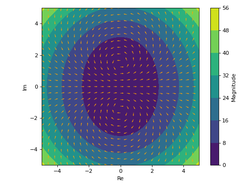
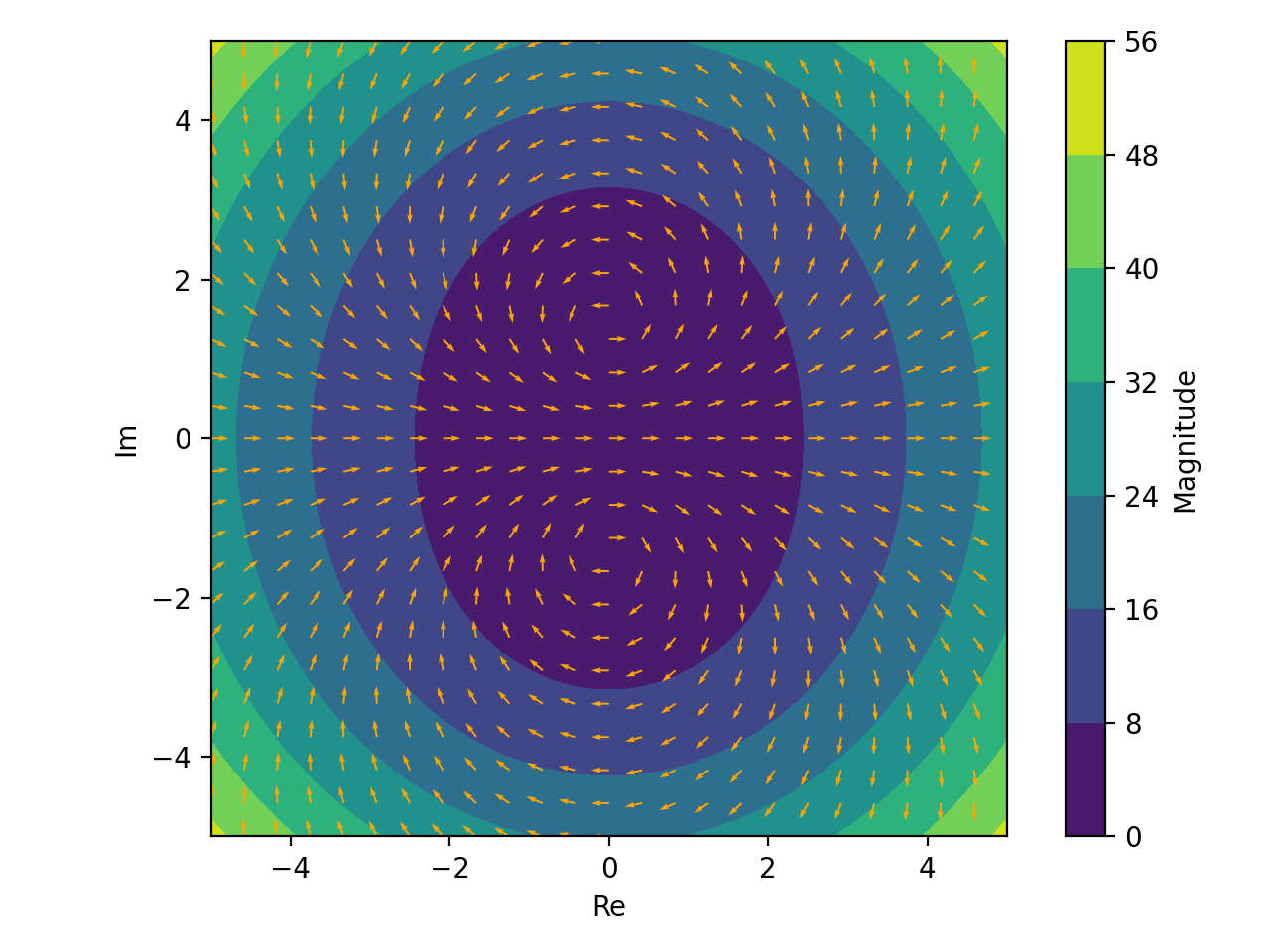
Quivers plot with normalize lengths and a contour plot in background representing the vector’s magnitude (a scalar field).

>>> expr = z**2 + 2
>>> plot_complex_vector(expr, (z, -5 - 5j, 5 + 5j),
...     quiver_kw=dict(color="orange"), normalize=True, grid=False)
Plot object containing:
[0]: contour: sqrt(4*(re(_x) - im(_y))**2*(re(_y) + im(_x))**2 + ((re(_x) - im(_y))**2 - (re(_y) + im(_x))**2 + 2)**2) for _x over (-5.0, 5.0) and _y over (-5.0, 5.0)
[1]: 2D vector series: [(re(_x) - im(_y))**2 - (re(_y) + im(_x))**2 + 2, 2*(re(_x) - im(_y))*(re(_y) + im(_x))] over (_x, -5.0, 5.0), (_y, -5.0, 5.0)

(Source code, png, hires.png, pdf)

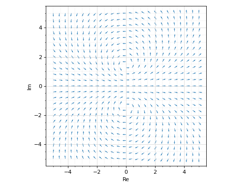
Only quiver plot with normalized lengths and solid color.

>>> plot_complex_vector(expr, (z, -5 - 5j, 5 + 5j),
...     scalar=False, use_cm=False, normalize=True)
Plot object containing:
[0]: 2D vector series: [(re(_x) - im(_y))**2 - (re(_y) + im(_x))**2 + 2, 2*(re(_x) - im(_y))*(re(_y) + im(_x))] over (_x, -5.0, 5.0), (_y, -5.0, 5.0)

(Source code, png, hires.png, pdf)

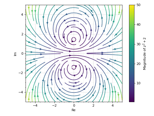
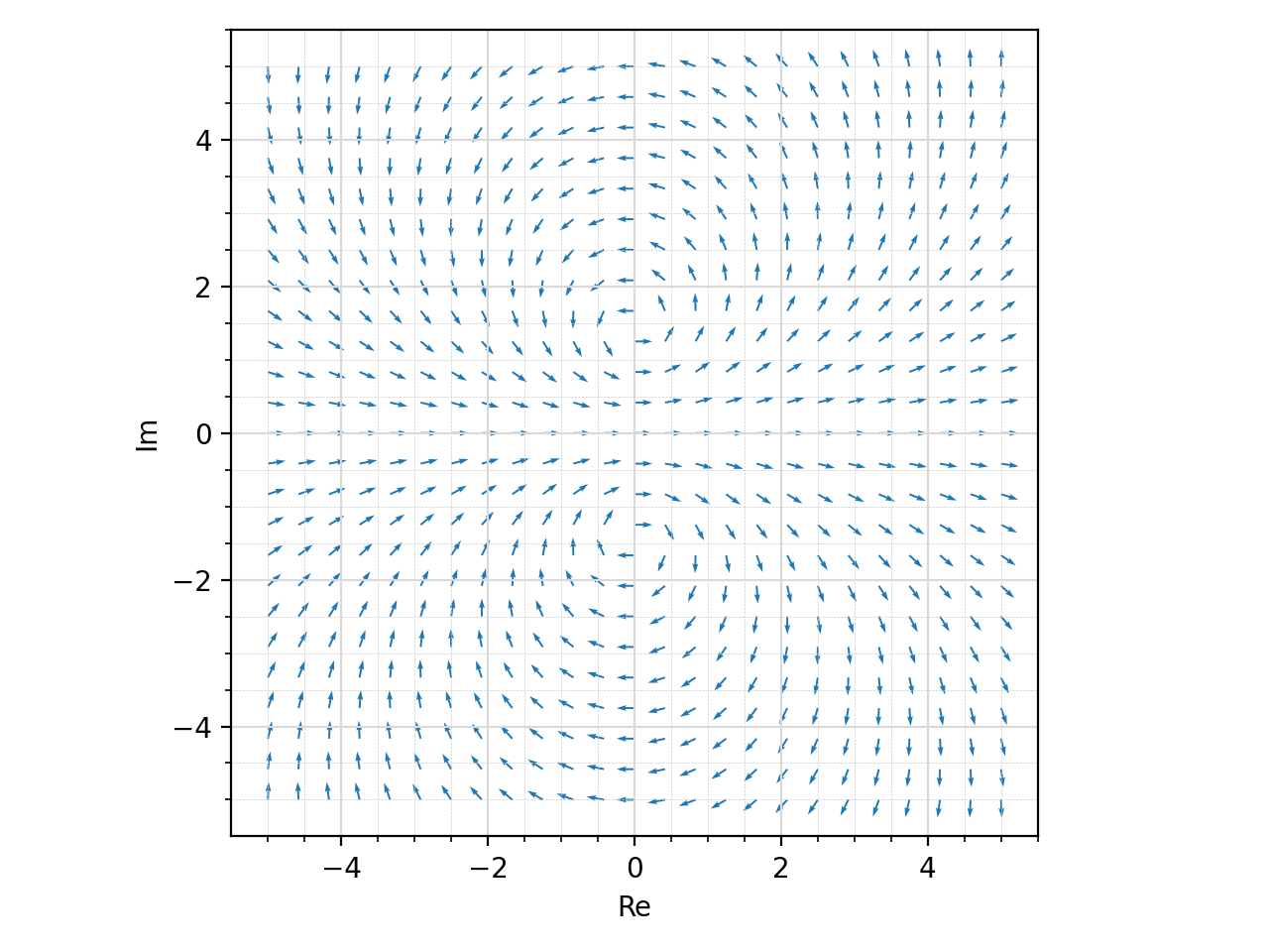
Only streamlines plot.

>>> plot_complex_vector(expr, (z, -5 - 5j, 5 + 5j),
...     "Magnitude of $%s$" % latex(expr),
...     scalar=False, streamlines=True)
Plot object containing:
[0]: 2D vector series: [(re(_x) - im(_y))**2 - (re(_y) + im(_x))**2 + 2, 2*(re(_x) - im(_y))*(re(_y) + im(_x))] over (_x, -5.0, 5.0), (_y, -5.0, 5.0)

(Source code, png, hires.png, pdf)

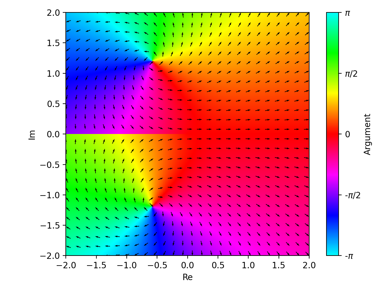
Overlay the quiver plot to a domain coloring plot. By setting n=26 (even number) in the complex vector plot, the quivers won’t to cross the branch cut.

>>> expr = z * log(2 * z) + 3
>>> p1 = plot_complex(expr, (z, -2-2j, 2+2j), grid=False, show=False)
>>> p2 = plot_complex_vector(expr, (z, -2-2j, 2+2j),
...      n=26, grid=False, scalar=False, use_cm=False, normalize=True,
...      quiver_kw={"color": "k", "pivot": "tip"}, show=False)
>>> (p1 + p2).show()
>>> (p1 + p2)
Plot object containing:
[0]: complex domain coloring: z*log(2*z) + 3 for re(z) over (-2.0, 2.0) and im(z) over (-2.0, 2.0)
[1]: 2D vector series: [(re(_x) - im(_y))*log(Abs(2*_x + 2*_y*I)) - (re(_y) + im(_x))*arg(_x + _y*I) + 3, (re(_x) - im(_y))*arg(_x + _y*I) + (re(_y) + im(_x))*log(Abs(2*_x + 2*_y*I))] over (_x, -2.0, 2.0), (_y, -2.0, 2.0)

(Source code, png, hires.png, pdf)

Interactive-widget plot. Refer to iplot documentation to learn more about the params dictionary.

from sympy import *
z, u = symbols("z u")
plot_complex_vector(
    log(gamma(u * z)), (z, -5 - 5j, 5 + 5j),
    params={u: (1, 0, 2)}, n=20,
    quiver_kw=dict(color="orange"), grid=False)