Vectors
- spb.vectors.plot_vector(*args, **kwargs)[source]
Plot a 2D or 3D vector field. By default, the aspect ratio of the plot is set to aspect=”equal”.
Typical usage examples are in the followings:
- Plotting a vector field with a single range.
plot(expr, range1, range2, range3 [optional], **kwargs)
- Plotting multiple vector fields with different ranges and custom labels.
plot((expr1, range1, range2, range3 [optional], label1 [optional]), (expr2, range4, range5, range6 [optional], label2 [optional]), **kwargs)
- Parameters
- args
- exprVector, or Matrix/list/tuple with 2 or 3 elements
Represents the vector to be plotted. It can be a:
Vector from the sympy.vector module or from the sympy.physics.mechanics module.
Matrix/list/tuple with 2 (or 3) symbolic elements.
list/tuple with 2 (or 3) numerical functions of 2 (or 3) variables.
Note: if a 3D symbolic vector is given with a list/tuple, it might happens that the internal algorithm thinks of it as a range. Therefore, 3D vectors should be given as a Matrix or as a Vector: this reduces ambiguities.
- ranges3-element tuples
Denotes the range of the variables. For example (x, -5, 5). For 2D vector plots, 2 ranges must be provided. For 3D vector plots, 3 ranges are needed.
- labelstr, optional
The name of the vector field to be eventually shown on the legend or colorbar. If none is provided, the string representation of the vector will be used.
- aspect(float, float) or str, optional
Set the aspect ratio of the plot. The value depends on the backend being used. Read that backend’s documentation to find out the possible values.
- backendPlot, optional
A subclass of Plot, which will perform the rendering. Default to MatplotlibBackend.
- contour_kwdict
A dictionary of keywords/values which is passed to the backend contour function to customize the appearance. Refer to the plotting library (backend) manual for more informations.
- labellist/tuple, optional
The label to be shown in the colorbar if
scalar=None. If not provided, the string representation of expr will be used.The number of labels must be equal to the number of series generated by the plotting function. For example:
if a scalar field and a quiver (or streamline) are shown simultaneously, then two labels must be provided;
if only a quiver (or streamline) is shown, then one label must be provided.
if two or more quivers (or streamlines) are shown, then two or more labels must be provided.
- n1, n2, n3int
Number of discretization points for the quivers or streamlines in the x/y/z-direction, respectively. Default to 25.
- nint or three-elements tuple (n1, n2, n3), optional
If an integer is provided, the ranges are sampled uniformly at n number of points. If a tuple is provided, it overrides n1, n2 and n3. Default to 25.
- ncint
Number of discretization points for the scalar contour plot. Default to 100.
- normalizebool
Default to False. If True, the vector field will be normalized, resulting in quivers having the same length. If
use_cm=True, the backend will color the quivers by the (pre-normalized) vector field’s magnitude. Note: only quivers will be affected by this option.- paramsdict
A dictionary mapping symbols to parameters. This keyword argument enables the interactive-widgets plot, which doesn’t support the adaptive algorithm (meaning it will use
adaptive=False). Learn more by reading the documentation ofiplot.- quiver_kwdict
A dictionary of keywords/values which is passed to the backend quivers- plotting function to customize the appearance. Refer to the plotting library (backend) manual for more informations.
- rendering_kwlist of dicts, optional
A list of dictionaries of keywords/values which is passed to the backend’s functions to customize the appearance.
The number of dictionaries must be equal to the number of series generated by the plotting function. For example:
if a scalar field and a quiver (or streamline) are shown simultaneously, then two dictionaries must be provided;
if only a quiver (or streamline) is shown, then one dictionary must be provided.
if two or more quivers (or streamlines) are shown, then two or more dictionaries must be provided.
Note that this will override
quiver_kw,stream_kw,contour_kw.- scalarboolean, Expr, None or list/tuple of 2 elements
Represents the scalar field to be plotted in the background of a 2D vector field plot. Can be:
True: plot the magnitude of the vector field. Only works when a single vector field is plotted.
False/None: do not plot any scalar field.
Expr: a symbolic expression representing the scalar field.
a numerical function of 2 variables supporting vectorization.
list/tuple: [scalar_expr, label], where the label will be shown on the colorbar. scalar_expr can be a symbolic expression or a numerical function of 2 variables supporting vectorization.
Default to True.
- showboolean
The default value is set to True. Set show to False and the function will not display the plot. The returned instance of the Plot class can then be used to save or display the plot by calling the save() and show() methods respectively.
- size(float, float), optional
A tuple in the form (width, height) to specify the size of the overall figure. The default value is set to None, meaning the size will be set by the backend.
- slicePlane, list, Expr
Plot the 3D vector field over the provided slice. It can be:
a Plane object from sympy.geometry module.
a list of planes.
an instance of
SurfaceOver2DRangeSeriesorParametricSurfaceSeries.a symbolic expression representing a surface of two variables.
The number of discretization points will be n1, n2, n3. Note that:
only quivers plots are supported with slices. Streamlines plots are unaffected.
n3 will only be used with planes parallel to xz or yz.
n1, n2, n3 doesn’t affect the slice if it is an instance of
SurfaceOver2DRangeSeriesorParametricSurfaceSeries.
- streamlinesboolean
Whether to plot the vector field using streamlines (True) or quivers (False). Default to False.
- stream_kwdict
A dictionary of keywords/values which is passed to the backend streamlines-plotting function to customize the appearance. Refer to the Notes section to learn more.
For 3D vector fields, by default the streamlines will start at the boundaries of the domain where the vectors are pointed inward. Depending on the vector field, this may results in too tight streamlines. Use the starts keyword argument to control the generation of streamlines:
starts=None: the default aforementioned behaviour.
starts=dict(x=x_list, y=y_list, z=z_list): specify the starting points of the streamlines.
starts=True: randomly create starting points inside the domain. In this setup we can set the number of starting point with npoints (default value to 200).
If 3D streamlines appears to be cut short inside the specified domain, try to increase max_prop (default value to 5000).
- titlestr, optional
Title of the plot. It is set to the latex representation of the expression, if the plot has only one expression.
- use_latexboolean, optional
Turn on/off the rendering of latex labels. If the backend doesn’t support latex, it will render the string representations instead.
- xlabelstr, optional
Label for the x-axis.
- ylabelstr, optional
Label for the y-axis.
- zlabelstr, optional
Label for the z-axis. Only available for 3D plots.
- xlim(float, float), optional
Denotes the x-axis limits, (min, max).
- ylim(float, float), optional
Denotes the y-axis limits, (min, max).
- zlim(float, float), optional
Denotes the z-axis limits, (min, max). Only available for 3D plots.
See also
iplot
Examples
>>> from sympy import symbols, sin, cos, Plane, Matrix, sqrt, latex
>>> from spb.vectors import plot_vector
>>> x, y, z = symbols('x, y, z')
Quivers plot of a 2D vector field with a contour plot in background representing the vector’s magnitude (a scalar field).
>>> v = [sin(x - y), cos(x + y)]
>>> plot_vector(v, (x, -3, 3), (y, -3, 3),
...     quiver_kw=dict(color="black", scale=30, headwidth=5),
...     contour_kw={"cmap": "Blues_r", "levels": 15},
...     grid=False, xlabel="x", ylabel="y")
Plot object containing:
[0]: contour: sqrt(sin(x - y)**2 + cos(x + y)**2) for x over (-3.0, 3.0) and y over (-3.0, 3.0)
[1]: 2D vector series: [sin(x - y), cos(x + y)] over (x, -3.0, 3.0), (y, -3.0, 3.0)
(Source code, png, hires.png, pdf)

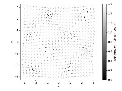
Quivers plot of a 2D vector field with no background scalar field, a custom label and normalized quiver lengths:
>>> plot_vector(
...     v, (x, -3, 3), (y, -3, 3),
...     label="Magnitude of $%s$" % latex([-sin(y), cos(x)]),
...     scalar=False, normalize=True,
...     quiver_kw={
...         "scale": 35, "headwidth": 4, "cmap": "gray",
...         "clim": [0, 1.6]},
...     grid=False, xlabel="x", ylabel="y")
Plot object containing:
[0]: contour: sqrt(sin(x - y)**2 + cos(x + y)**2) for x over (-3.0, 3.0) and y over (-3.0, 3.0)
[1]: 2D vector series: [sin(x - y), cos(x + y)] over (x, -3.0, 3.0), (y, -3.0, 3.0)
(Source code, png, hires.png, pdf)
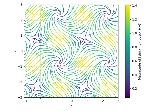
Streamlines plot of a 2D vector field with no background scalar field, and a custom label:
>>> plot_vector(v, (x, -3, 3), (y, -3, 3),
...     streamlines=True, scalar=None,
...     stream_kw={"density": 1.5},
...     label="Magnitude of %s" % str(v), xlabel="x", ylabel="y")
Plot object containing:
[0]: 2D vector series: [sin(x - y), cos(x + y)] over (x, -3.0, 3.0), (y, -3.0, 3.0)
(Source code, png, hires.png, pdf)
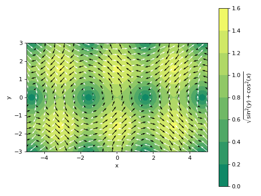
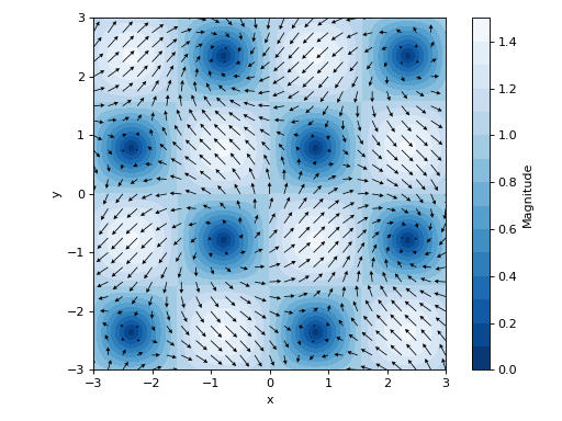
Plot multiple 2D vectors fields, setting a background scalar field to be the magnitude of the first vector. Also, apply custom rendering options to all data series.
>>> scalar_expr = sqrt((-sin(y))**2 + cos(x)**2)
>>> plot_vector([-sin(y), cos(x)], [2 * y, x], (x, -5, 5), (y, -3, 3),
...     n=20, legend=True, grid=False, xlabel="x", ylabel="y",
...     scalar=[scalar_expr, "$%s$" % latex(scalar_expr)],
...     rendering_kw=[
...         {"cmap": "summer"}, # to the contour
...         {"color": "k"},     # to the first quiver
...         {"color": "w"}      # to the second quiver
... ])
Plot object containing:
[0]: contour: sqrt(sin(y)**2 + cos(x)**2) for x over (-5.0, 5.0) and y over (-3.0, 3.0)
[1]: 2D vector series: [-sin(y), cos(x)] over (x, -5.0, 5.0), (y, -3.0, 3.0)
[2]: 2D vector series: [y, x] over (x, -5.0, 5.0), (y, -3.0, 3.0)
(Source code, png, hires.png, pdf)
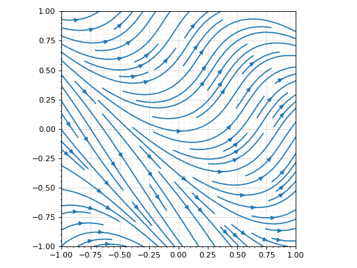
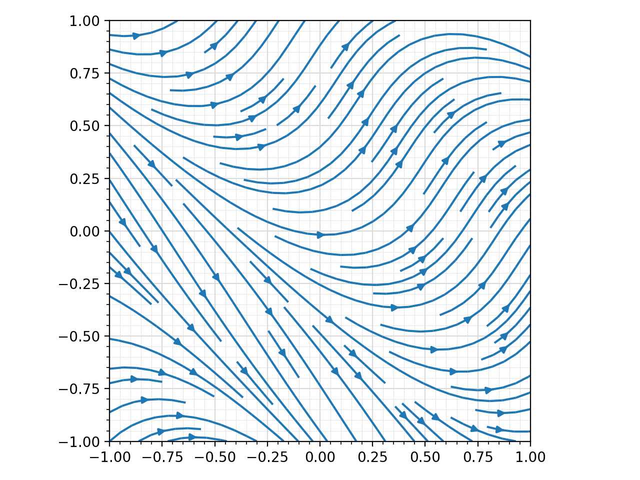
Plotting a the streamlines of a 2D vector field defined with numerical functions instead of symbolic expressions:
>>> import numpy as np
>>> f = lambda x, y: np.sin(2 * x + 2 * y)
>>> fx = lambda x, y: np.cos(f(x, y))
>>> fy = lambda x, y: np.sin(f(x, y))
>>> plot_vector([fx, fy], ("x", -1, 1), ("y", -1, 1),
...     streamlines=True, scalar=False, use_cm=False)
(Source code, png, hires.png, pdf)

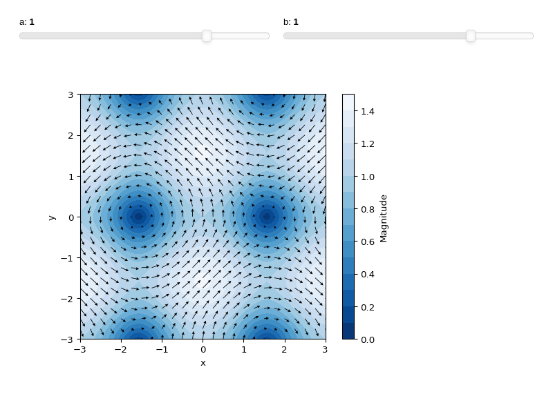
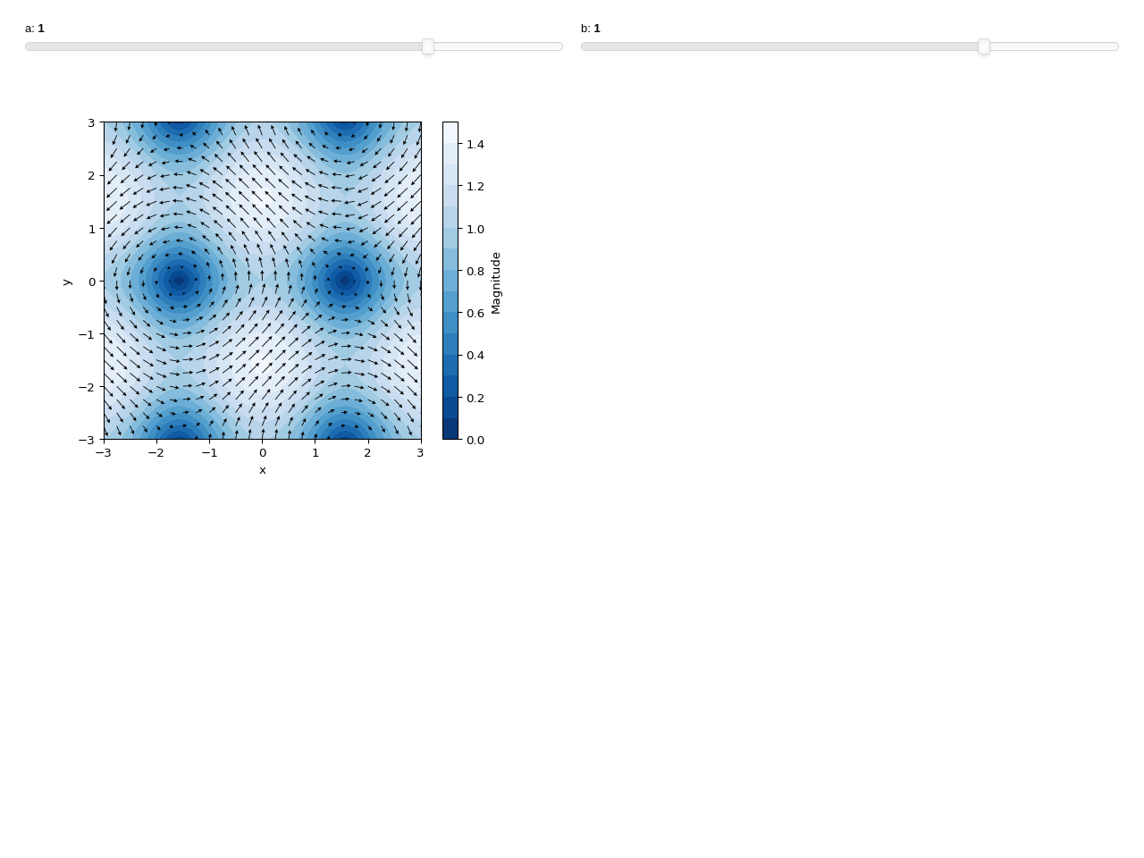
Interactive-widget 2D vector plot. Refer to
iplotdocumentation to learn more about theparamsdictionary.from sympy import * from spb import * x, y, a, b = symbols("x, y, a, b") v = [-sin(a * y), cos(b * x)] plot_vector( v, (x, -3, 3), (y, -3, 3), params={a: (1, -2, 2), b: (1, -2, 2)}, quiver_kw=dict(color="black", scale=30, headwidth=5), contour_kw={"cmap": "Blues_r", "levels": 15}, grid=False, xlabel="x", ylabel="y", use_latex=False)
(Source code, small.png, large.png, html, pdf)

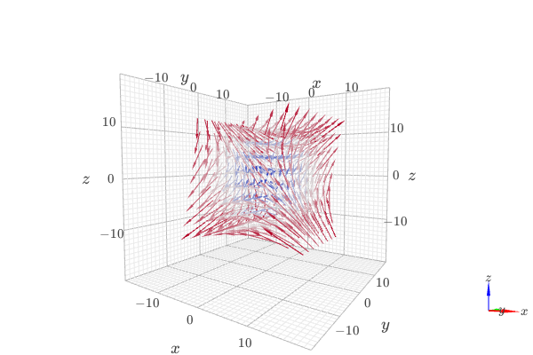
3D vector field.
from sympy import *
from spb import *
var("x:z")
plot_vector([z, y, x], (x, -10, 10), (y, -10, 10), (z, -10, 10),
    backend=KB, n=8, xlabel="x", ylabel="y", zlabel="z",
    quiver_kw={"scale": 0.5, "line_width": 0.1, "head_size": 10})
(Source code, small.png, large.png, html, pdf)

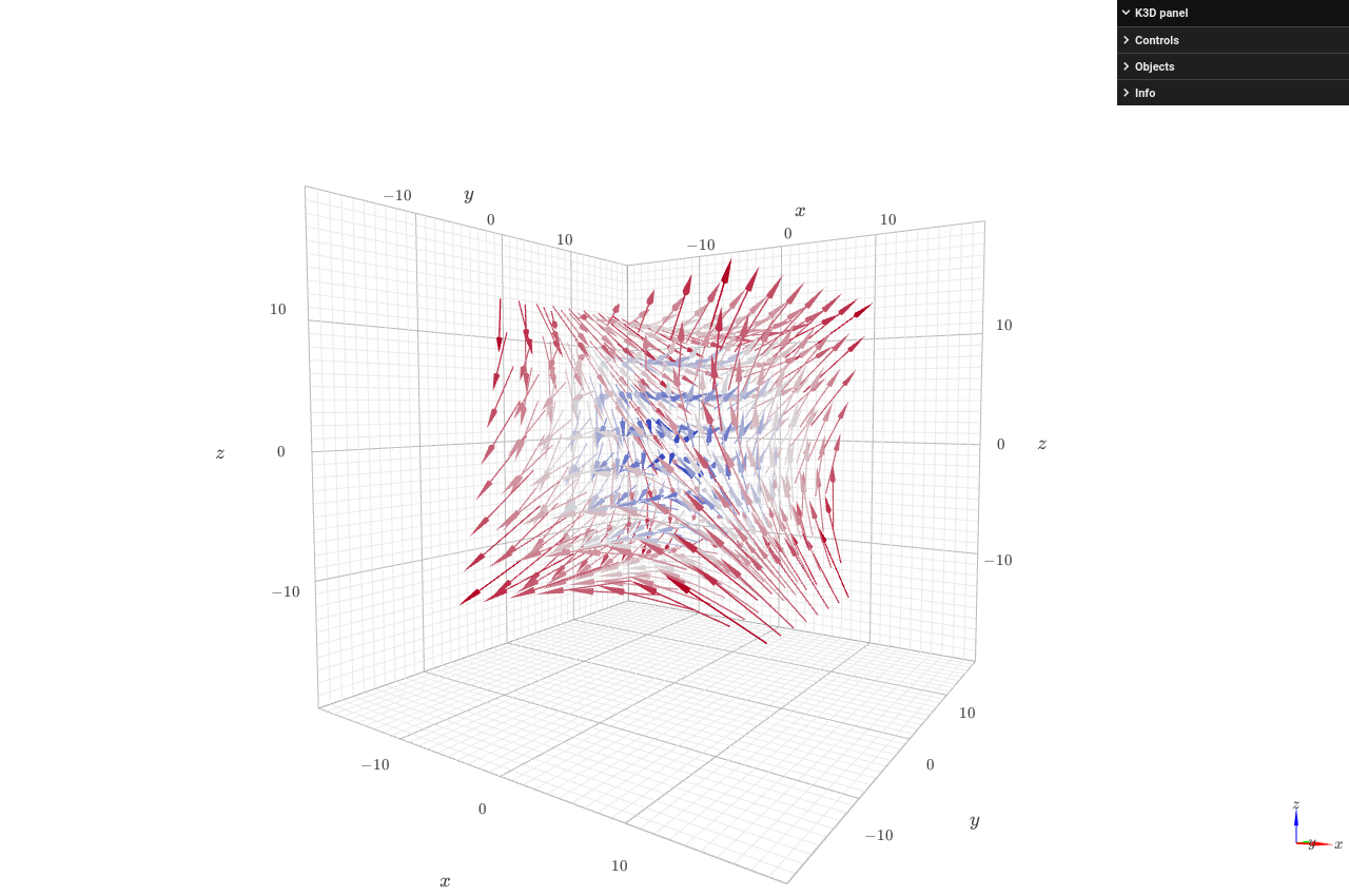
3D vector field with 3 orthogonal slice planes.
from sympy import *
from spb import *
var("x:z")
plot_vector([z, y, x], (x, -10, 10), (y, -10, 10), (z, -10, 10),
    backend=KB, n=8, use_cm=False, grid=False,
    xlabel="x", ylabel="y", zlabel="z",
    quiver_kw={"scale": 0.25, "line_width": 0.1, "head_size": 10},
    slice=[
        Plane((-10, 0, 0), (1, 0, 0)),
        Plane((0, 10, 0), (0, 2, 0)),
        Plane((0, 0, -10), (0, 0, 1))])
(Source code, small.png, large.png, html, pdf)
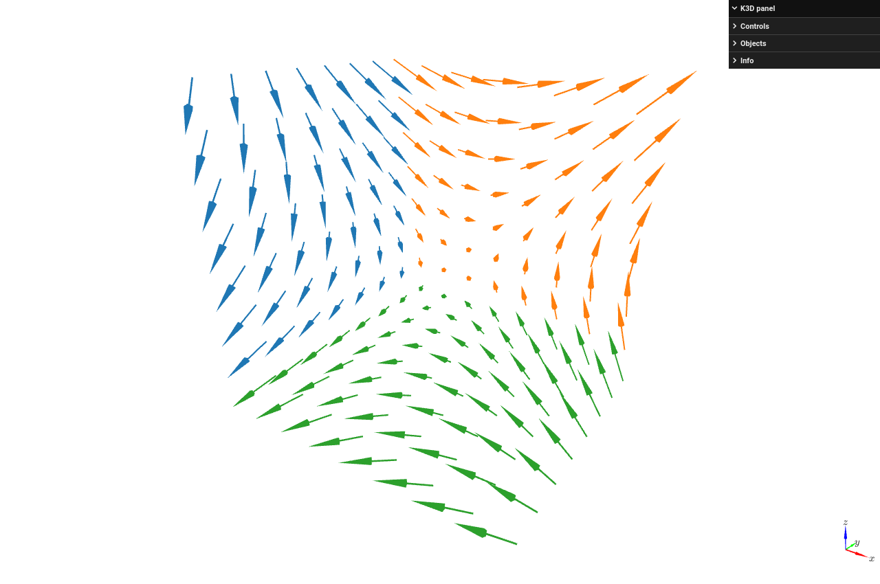
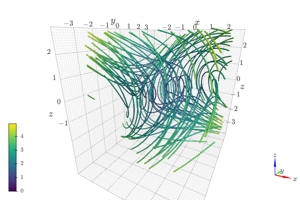
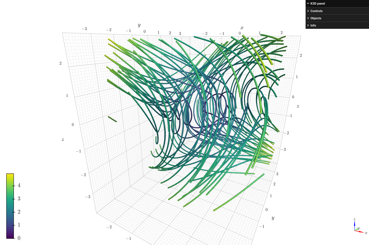
3D vector streamlines starting at a 300 random points:
from sympy import *
from spb import *
import k3d
var("x:z")
plot_vector(Matrix([z, -x, y]), (x, -3, 3), (y, -3, 3), (z, -3, 3),
    backend=KB, n=40, streamlines=True,
    stream_kw=dict(
        starts=True,
        npoints=400,
        width=0.025,
        color_map=k3d.colormaps.matplotlib_color_maps.viridis
    ),
    xlabel="x", ylabel="y", zlabel="z")
(Source code, small.png, large.png, html, pdf)

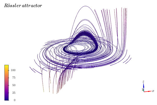
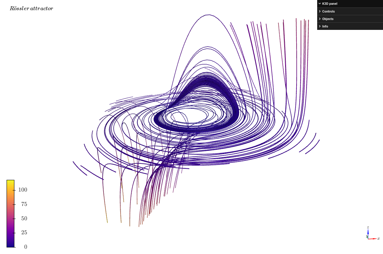
3D vector streamlines starting at the XY plane. Note that the number of discretization points of the plane controls the numbers of streamlines.
from sympy import *
from spb import *
import k3d
var("x:z")
u = -y - z
v = x + y / 5
w = S(1) / 5 + (x - S(5) / 2) * z
s = 10 # length of the cubic discretization volume
# create an XY plane with n discretization points along each direction
n = 8
p1 = plot_geometry(
    Plane((0, 0, 0), (0, 0, 1)), (x, -s, s), (y, -s, s), (z, -s, s),
    n1=n, n2=n, show=False)
# extract the coordinates of the starting points for the streamlines
xx, yy, zz = p1[0].get_data()
# streamlines plot
plot_vector(Matrix([u, v, w]), (x, -s, s), (y, -s, s), (z, -s, s),
    backend=KB, n=40, streamlines=True, grid=False,
    stream_kw=dict(
        starts=dict(x=xx, y=yy, z=zz),
        npoints=200,
        width=0.025,
        color_map=k3d.colormaps.matplotlib_color_maps.plasma
    ),
    title="Rössler \, attractor", xlabel="x", ylabel="y", zlabel="z")
(Source code, small.png, large.png, html, pdf)

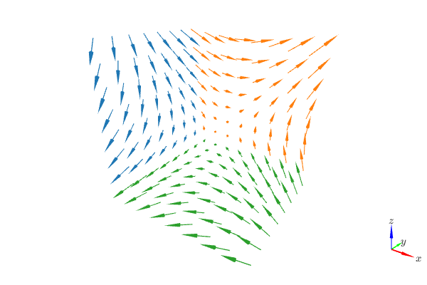
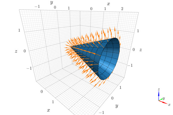
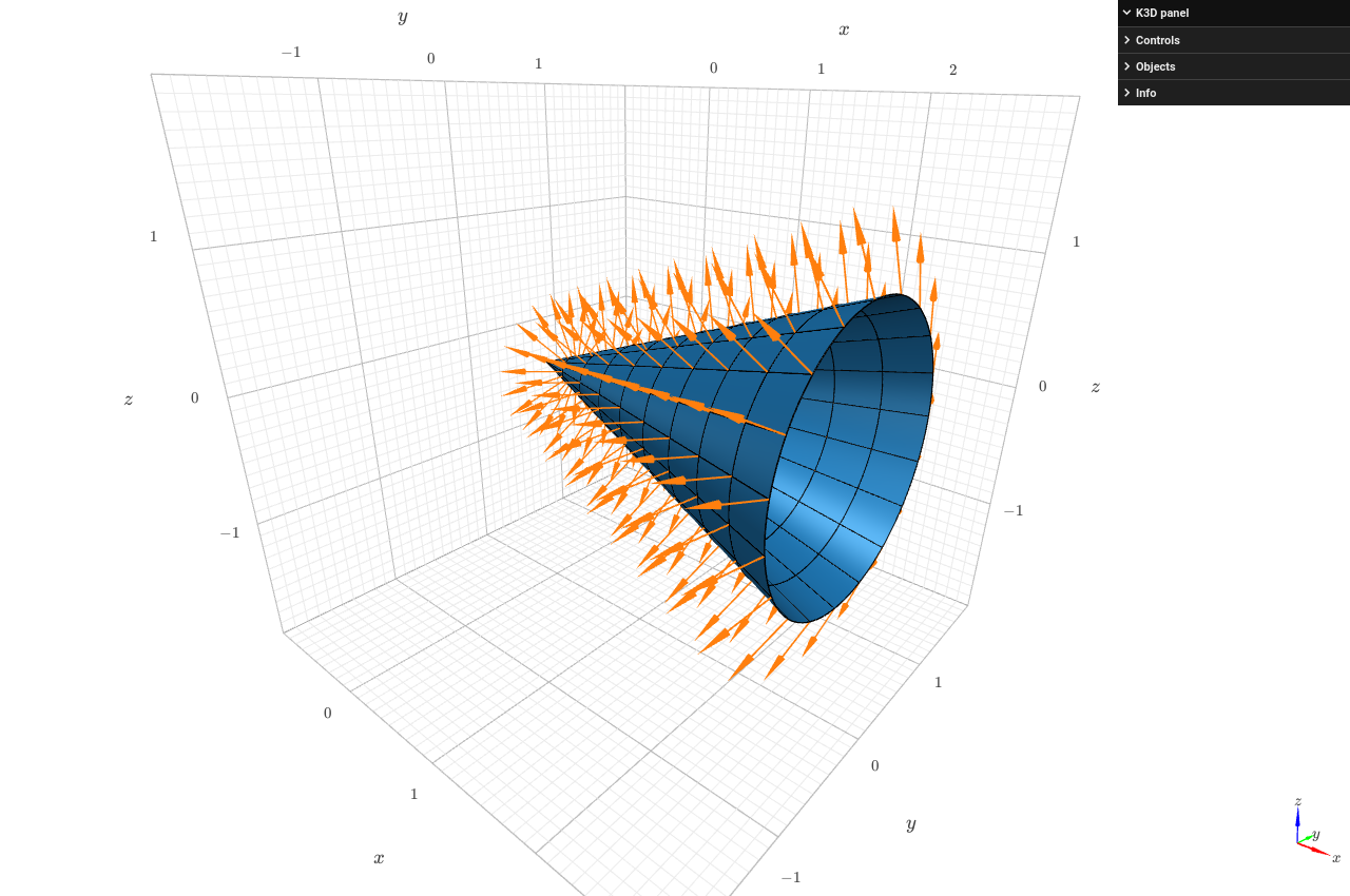
Visually verify the normal vector to a circular cone surface. The following steps are executed:
compute the normal vector to a circular cone surface. This will be the vector field to be plotted.
plot the cone surface for visualization purposes (use high number of discretization points).
plot the cone surface that will be used to slice the vector field (use a low number of discretization points). The data series associated to this plot will be used in the
slicekeyword argument in the next step.plot the sliced vector field.
combine the plots of step 4 and 2 to get a nice visualization.
from sympy import tan, cos, sin, pi, symbols
from spb import plot3d_parametric_surface, plot_vector, KB
from sympy.vector import CoordSys3D, gradient

u, v = symbols("u, v")
N = CoordSys3D("N")
i, j, k = N.base_vectors()
xn, yn, zn = N.base_scalars()

t = 0.35    # half-cone angle in radians
expr = -xn**2 * tan(t)**2 + yn**2 + zn**2    # cone surface equation
g = gradient(expr)
n = g / g.magnitude()    # unit normal vector
n1, n2 = 10, 20 # number of discretization points for the vector field

# cone surface for visualization (high number of discretization points)
p1 = plot3d_parametric_surface(
    u / tan(t), u * cos(v), u * sin(v), (u, 0, 1), (v, 0 , 2*pi),
    {"opacity": 1}, backend=KB, show=False, wireframe=True,
    wf_n1=n1, wf_n2=n2, wf_rendering_kw={"width": 0.004})
# cone surface to discretize vector field (low numb of discret points)
p2 = plot3d_parametric_surface(
    u / tan(t), u * cos(v), u * sin(v), (u, 0, 1), (v, 0 , 2*pi),
    n1=n1, n2=n2, show=False)
# plot vector field on over the surface of the cone
p3 = plot_vector(
    n, (xn, -5, 5), (yn, -5, 5), (zn, -5, 5), slice=p2[0],
    backend=KB, use_cm=False, show=False,
    quiver_kw={"scale": 0.5, "pivot": "tail"})
(p1 + p3).show()
(Source code, small.png, large.png, html, pdf)
