1 - Combining plots
Let’s understand what happens when a plot command is executed:
from sympy import *
from spb import *
var("x")
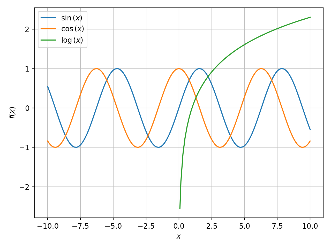
p = plot(sin(x), cos(x), log(x), backend=MB)
(Source code, png, hires.png, pdf)
The plot function is going to loop over the provided arguments: it will create
and store one data series for each expression. So, in the previous example
p contains 3 data series. Once the data series are created, they will be
used by the backend (the wrapper to the plotting library) to generate
numerical data.
Effectively, p is a container of data series. We can quickly visualize
them by printing the plot object:
>>> print(p)
Plot object containing:
[0]: cartesian line: sin(x) for x over (-10.0, 10.0)
[1]: cartesian line: cos(x) for x over (-10.0, 10.0)
[2]: cartesian line: log(x) for x over (-10.0, 10.0)
We can retrieve a list containing all data series from a plot object by
calling the series attribute:
p.series
Alternatively, we can retrieve a single data series by indexing the plot object:
>>> print(p[0])
cartesian line: sin(x) for x over (-10.0, 10.0)
We can combine multiple plots together in three ways:
summing them up: this will create a new plot containing all data series from all initial plots. For example:
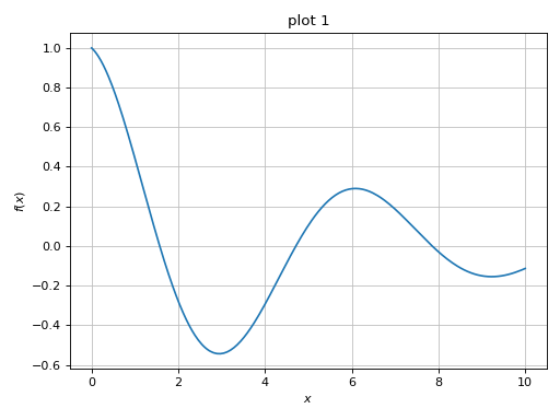
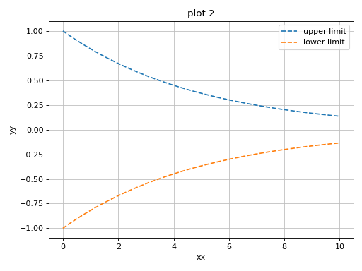
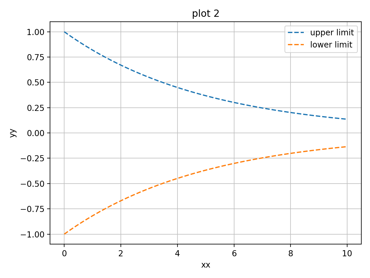
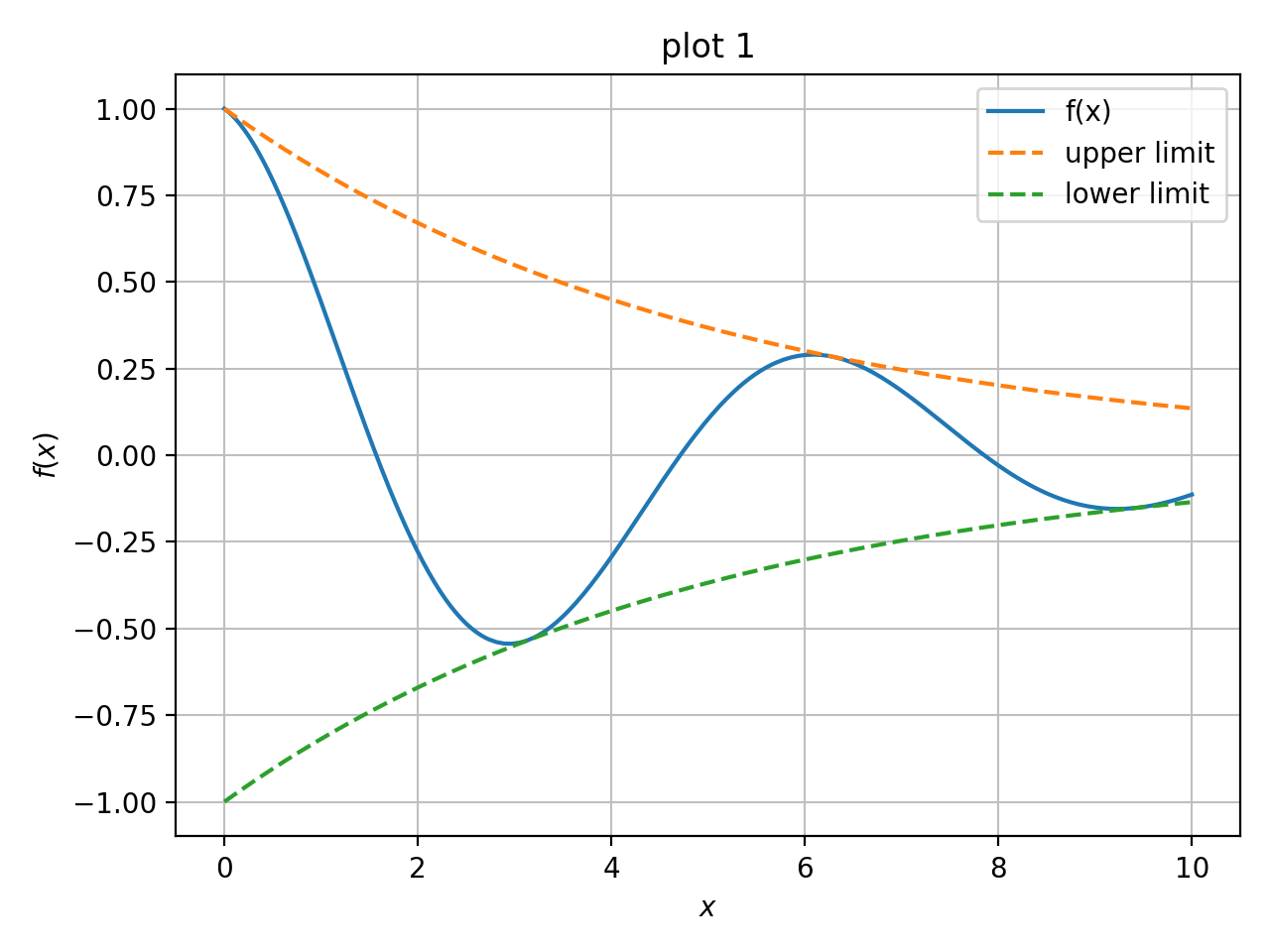
c = S(2) / 10
p1 = plot(cos(x) * exp(-c * x), (x, 0, 10), "f(x)", title="plot 1")
p2 = plot(
    (exp(-c * x), "upper limit"),
    (-exp(-c * x), "lower limit"), (x, 0, 10), {"linestyle": "--"},
    title="plot 2", xlabel="xx", ylabel="yy")
And then:
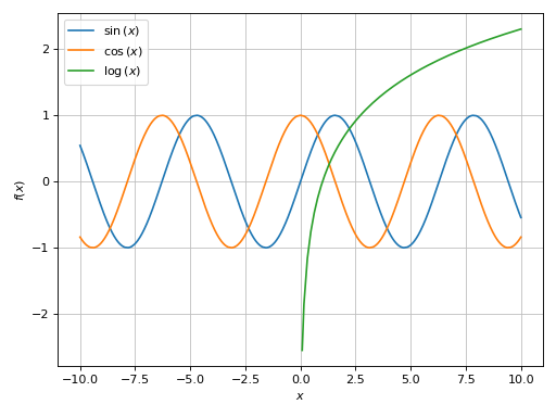
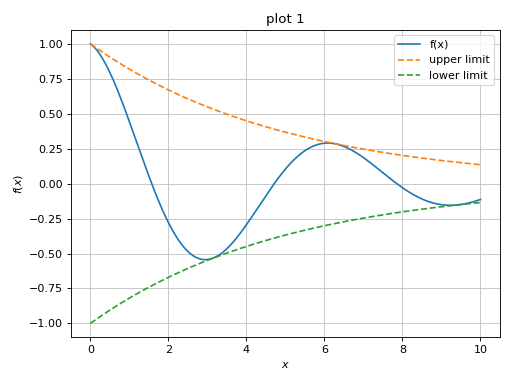
p3 = p1 + p2
p3.show()
# or more quickly: (p1 + p2).show()
(Source code, png, hires.png, pdf)

Note that the final plot uses the keyword arguments of the left-most plot in the summation. In the previous example, the resulting plot has the title of
p1. Now, let’s sum them up in a different order:(p2 + p1).show()
(Source code, png, hires.png, pdf)
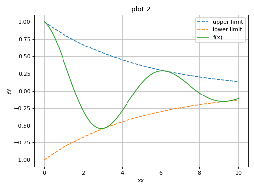
Here, the resulting plot is using the title and axis labels of
p2.We can use the
extendmethod to achieve the same goal as before:p1.extend(p2) p1.show()
(Source code, png, hires.png, pdf)
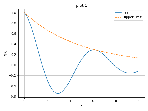
using the
appendmethod to append one specific data series from one plot object to another. For example:>>> p1 = plot(cos(x) * exp(-c * x), (x, 0, 10), "f(x)", ... title="plot 1", show=False) >>> p2 = plot( ... (exp(-c * x), "upper limit"), ... (-exp(-c * x), "lower limit"), (x, 0, 10), {"linestyle": "--"}, ... title="plot 2", xlabel="xx", ylabel="yy", show=False) >>> p1.append(p2[0]) >>> print(p1) Plot object containing: [0]: cartesian line: exp(-x/5)*cos(x) for x over (0.0, 10.0) [1]: cartesian line: exp(-x/5) for x over (0.0, 10.0) >>> p1.show()
(Source code, png, hires.png, pdf)