3D general plotting
NOTE:
For technical reasons, all interactive-widgets plots in this documentation are
created using Holoviz’s Panel. Often, they will ran just fine with ipywidgets
too. However, if a specific example uses the param library, then users
will have to modify the params dictionary in order to make it work with
ipywidgets. Refer to Interactive module for more information.
- spb.functions.plot3d(*args, **kwargs)[source]
Plots a 3D surface plot.
Typical usage examples are in the followings:
- Plotting a single expression.
plot3d(expr, range_x, range_y, **kwargs)
- Plotting multiple expressions with the same ranges.
plot3d(expr1, expr2, range_x, range_y, **kwargs)
- Plotting multiple expressions with different ranges.
plot3d((expr1, range_x1, range_y1), (expr2, range_x2, range_y2), …, **kwargs)
- Plotting multiple expressions with custom labels and rendering options.
plot3d((expr1, range_x1, range_y1, label1, rendering_kw1), (expr2, range_x2, range_y2, label2, rendering_kw2), …, **kwargs)
Note: it is important to specify at least the
range_x, otherwise the function might create a rotated plot.- Parameters:
- args
- exprExpr
Expression representing the function of two variables to be plotted. The expression representing the function of two variables to be plotted. It can be a:
Symbolic expression.
Numerical function of two variable, supporting vectorization. In this case the following keyword arguments are not supported:
params.
- range_x: (symbol, min, max)
A 3-tuple denoting the range of the x variable. Default values: min=-10 and max=10.
- range_y: (symbol, min, max)
A 3-tuple denoting the range of the y variable. Default values: min=-10 and max=10.
- labelstr, optional
The label to be shown in the colorbar. If not provided, the string representation of
exprwill be used.- rendering_kwdict, optional
A dictionary of keywords/values which is passed to the backend’s function to customize the appearance of surfaces. Refer to the plotting library (backend) manual for more informations.
- adaptivebool, optional
The default value is set to
False, which uses a uniform sampling strategy with number of discretization pointsn1andn2along the x and y directions, respectively.Set adaptive to
Trueto use the adaptive algorithm implemented in [1] to create smooth plots. Useadaptive_goalandloss_fnto further customize the output.- adaptive_goalcallable, int, float or None
Controls the “smoothness” of the evaluation. Possible values:
None(default): it will use the following goal:lambda l: l.loss() < 0.01number (int or float). The lower the number, the more evaluation points. This number will be used in the following goal:
lambda l: l.loss() < numbercallable: a function requiring one input element, the learner. It must return a float number. Refer to [1] for more information.
- backendPlot, optional
A subclass of
Plot, which will perform the rendering. Default toMatplotlibBackend.- colorbarboolean, optional
Show/hide the colorbar. Default to True (colorbar is visible). Only works when
use_cm=True.- color_funccallable, optional
Define the surface color mapping when
use_cm=True. It can either be:A numerical function of 3 variables, x, y, z (the points computed by the internal algorithm) supporting vectorization.
A symbolic expression having at most as many free symbols as
expr.None: the default value (color mapping applied to the z-value of the surface).
- force_real_evalboolean, optional
Default to False, with which the numerical evaluation is attempted over a complex domain, which is slower but produces correct results. Set this to True if performance is of paramount importance, but be aware that it might produce wrong results. It only works with
adaptive=False.- is_polarboolean, optional
Default to False. If True, requests a polar discretization. In this case,
range_xrepresents the radius,range_yrepresents the angle.- labelstr or list/tuple, optional
The label to be shown in the colorbar. If not provided, the string representation of
exprwill be used. The number of labels must be equal to the number of expressions.- legendbool, optional
Show/hide the legend. Default to None (the backend determines when it is appropriate to show it). Only works when
use_cm=False.- loss_fncallable or None
The loss function to be used by the adaptive learner. Possible values:
None(default): it will use thedefault_lossfrom theadaptivemodule.callable : Refer to [1] for more information. Specifically, look at
adaptive.learner.learnerNDto find more loss functions.
- n1, n2int, optional
n1andn2set the number of discretization points along the x and y ranges, respectively. Default value to 100.- nint or two-elements tuple (n1, n2), optional
If an integer is provided, the x and y ranges are sampled uniformly at
nof points. If a tuple is provided, it overridesn1andn2.- paramsdict
A dictionary mapping symbols to parameters. This keyword argument enables the interactive-widgets plot, which doesn’t support the adaptive algorithm (meaning it will use
adaptive=False). Learn more by reading the documentation of the interactive sub-module.- rendering_kwdict or list of dicts, optional
A dictionary of keywords/values which is passed to the backend’s function to customize the appearance of surfaces. Refer to the plotting library (backend) manual for more informations. If a list of dictionaries is provided, the number of dictionaries must be equal to the number of expressions.
- showbool, optional
The default value is set to
True. Set show toFalseand the function will not display the plot. The returned instance of the Plot class can then be used to save or display the plot by calling thesave()andshow()methods respectively.- size(float, float), optional
A tuple in the form (width, height) to specify the size of the overall figure. The default value is set to
None, meaning the size will be set by the backend.- titlestr, optional
Title of the plot. It is set to the latex representation of the expression, if the plot has only one expression.
- tx, ty, tzcallable, optional
Apply a numerical function to the discretized domain in the x, y and z direction, respectively.
- use_cmboolean, optional
If True, apply a color map to the surface. If False, solid colors will be used instead. Default to False.
- use_latexboolean, optional
Turn on/off the rendering of latex labels. If the backend doesn’t support latex, it will render the string representations instead.
- wireframeboolean, optional
Enable or disable a wireframe over the surface. Depending on the number of wireframe lines (see
wf_n1andwf_n2), activating this option might add a considerable overhead during the plot’s creation. Default to False (disabled).- wf_n1, wf_n2int, optional
Number of wireframe lines along the x and y ranges, respectively. Default to 10. Note that increasing this number might considerably slow down the plot’s creation.
- wf_npointint or None, optional
Number of discretization points for the wireframe lines. Default to None, meaning that each wireframe line will have
n1orn2number of points, depending on the line direction.- wf_rendering_kwdict, optional
A dictionary of keywords/values which is passed to the backend’s function to customize the appearance of wireframe lines.
- xlabel, ylabel, zlabelstr, optional
Labels for the x-axis or y-axis or z-axis, respectively.
- xlim, ylim(float, float), optional
Denotes the x-axis limits or y-axis limits,
(min, max), visible in the chart. Note that the function is still being evaluate overrange_xandrange_y.- zlim(float, float), optional
Denotes the z-axis limits,
(min, max), visible in the chart.
See also
plot3d_parametric_list,plot3d_parametric_surface,plot3d_sphericalplot3d_revolution,plot3d_implicit,plot3d_list,plot_contour
References
Examples
Note: for documentation purposes, the following examples uses Matplotlib. However, Matplotlib’s 3D capabilities are rather limited. Consider running these examples with a different backend (hence, modify the
rendering_kwandwf_rendering_kwto pass the correct options to the backend).>>> from sympy import symbols, cos, sin, pi, exp >>> from spb import plot3d >>> x, y = symbols('x y')
Single plot with Matplotlib:
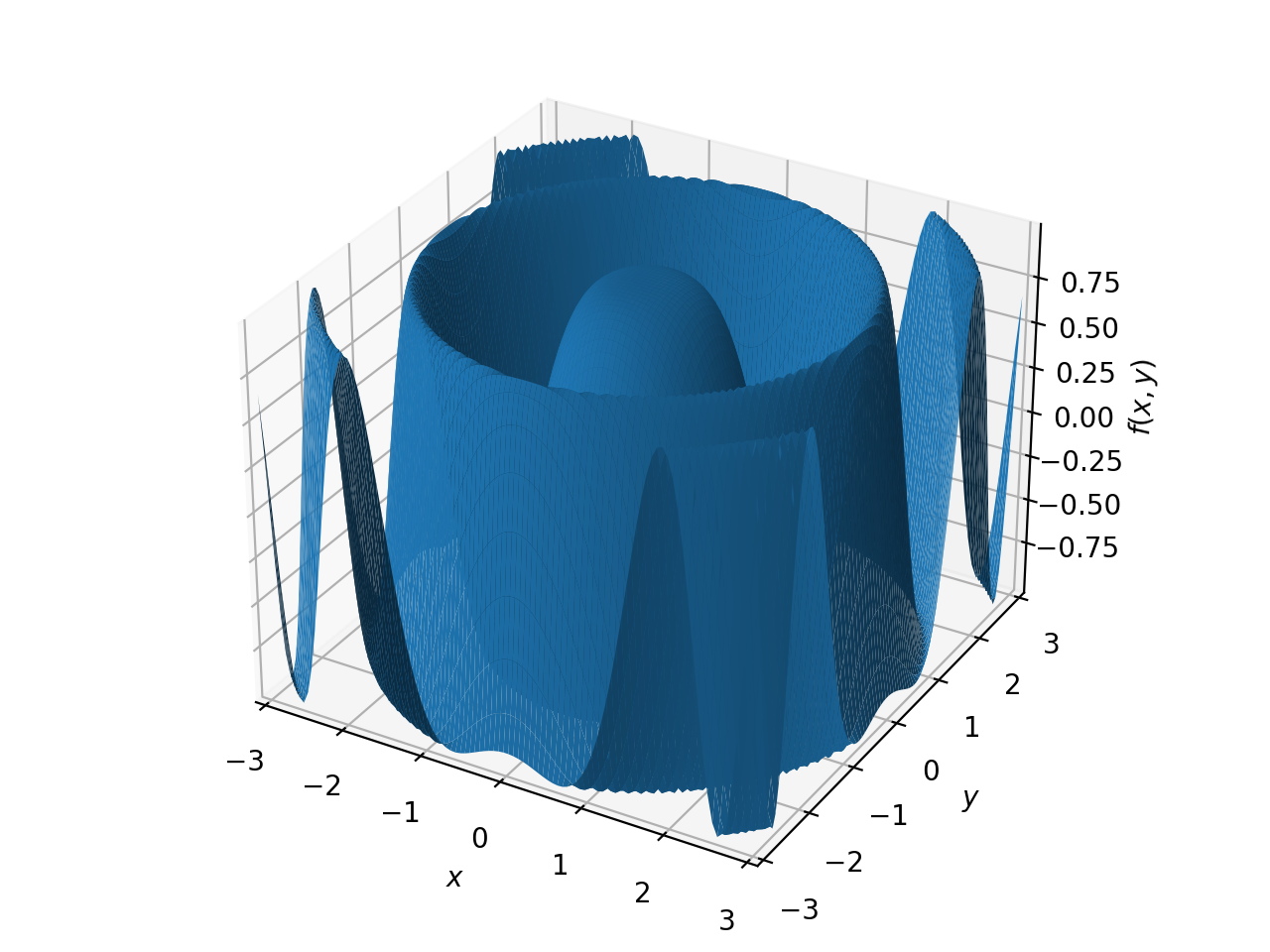
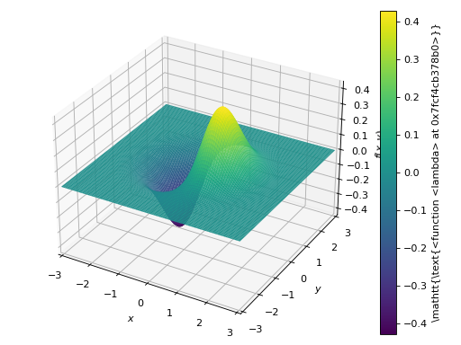
>>> plot3d(cos((x**2 + y**2)), (x, -3, 3), (y, -3, 3))
Plot object containing:
[0]: cartesian surface: cos(x**2 + y**2) for x over (-3.0, 3.0) and y over (-3.0, 3.0)
(
Source code,png,hires.png,pdf)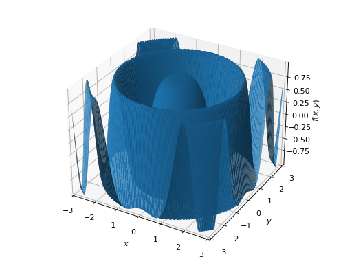
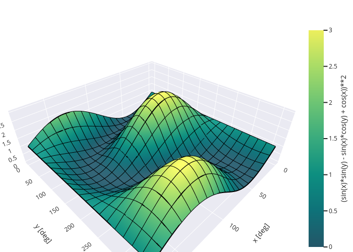
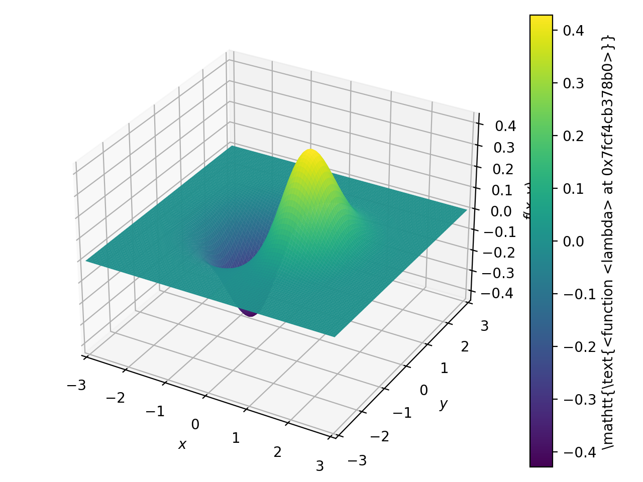
Single plot with Plotly, illustrating how to apply:
a color map: by default, it will map colors to the z values.
wireframe lines to better understand the discretization and curvature.
transformation to the discretized ranges in order to convert radians to degrees.
custom aspect ratio with Plotly.
from sympy import symbols, sin, cos, pi
from spb import plot3d, PB
import numpy as np
x, y = symbols("x, y")
expr = (cos(x) + sin(x) * sin(y) - sin(x) * cos(y))**2
plot3d(
    expr, (x, 0, pi), (y, 0, 2 * pi), backend=PB, use_cm=True,
    tx=np.rad2deg, ty=np.rad2deg, wireframe=True, wf_n1=20, wf_n2=20,
    xlabel="x [deg]", ylabel="y [deg]",
    aspect=dict(x=1.5, y=1.5, z=0.5))
(Source code, png, pdf, html)
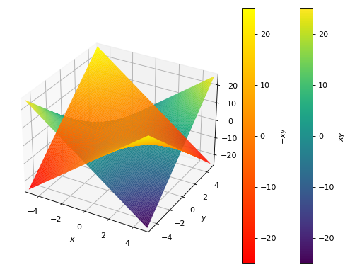
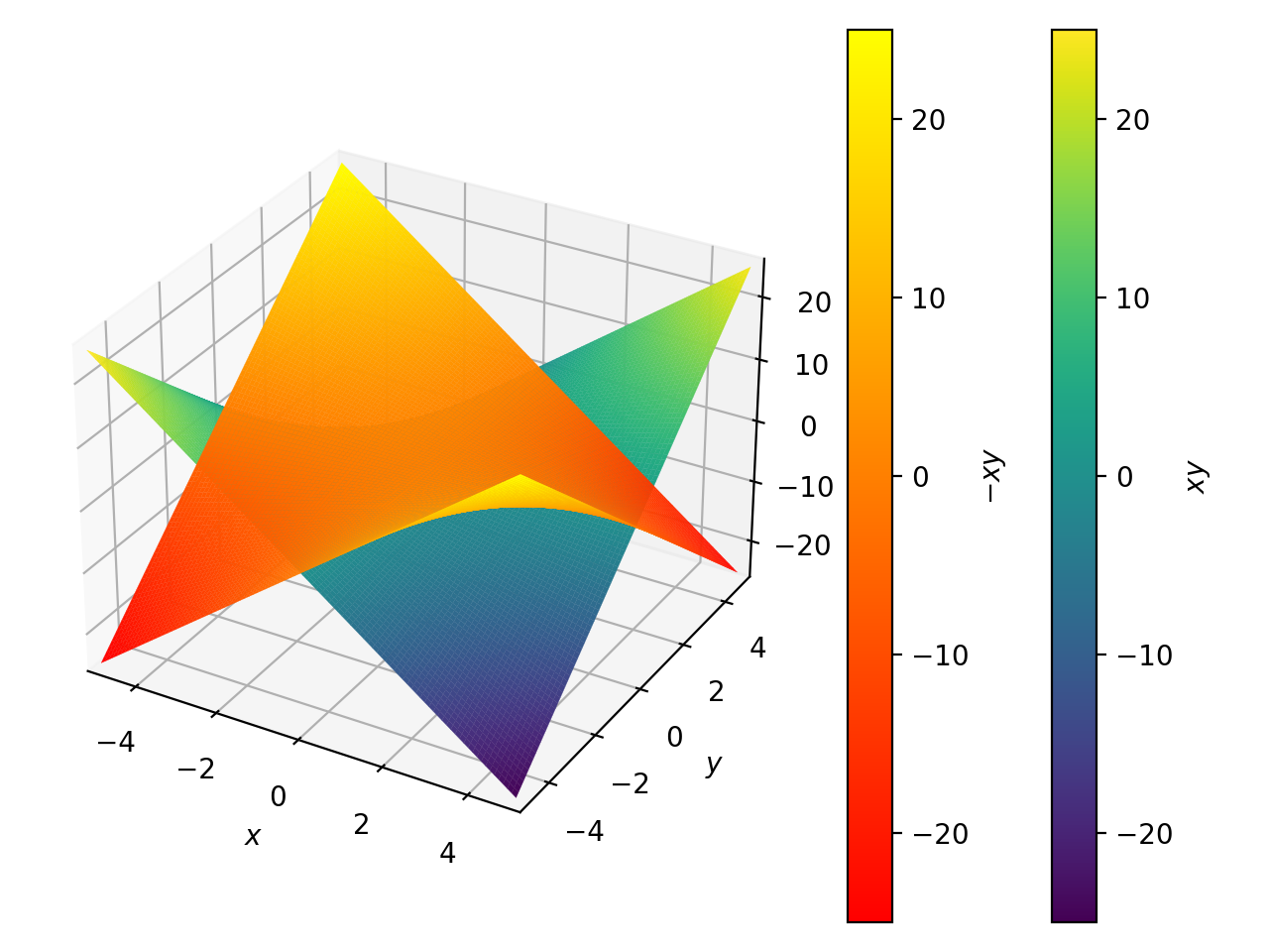
Multiple plots with same range using color maps. By default, colors are mapped to the z values:
>>> plot3d(x*y, -x*y, (x, -5, 5), (y, -5, 5), use_cm=True)
Plot object containing:
[0]: cartesian surface: x*y for x over (-5.0, 5.0) and y over (-5.0, 5.0)
[1]: cartesian surface: -x*y for x over (-5.0, 5.0) and y over (-5.0, 5.0)
(
Source code,png,hires.png,pdf)
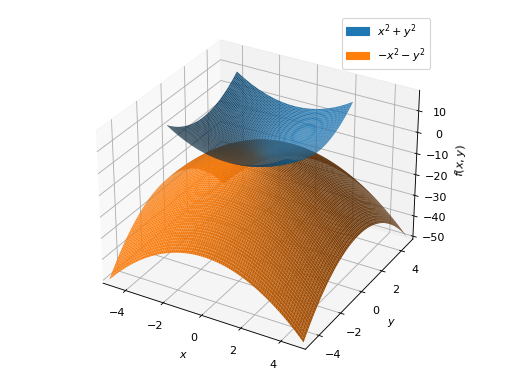
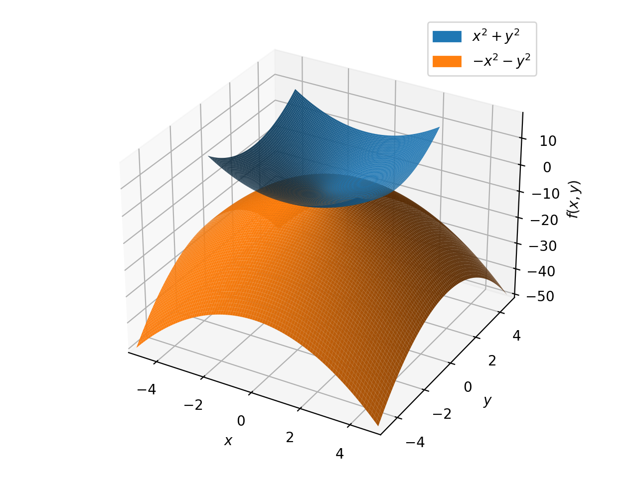
Multiple plots with different ranges and solid colors.
>>> f = x**2 + y**2
>>> plot3d((f, (x, -3, 3), (y, -3, 3)),
...     (-f, (x, -5, 5), (y, -5, 5)))
Plot object containing:
[0]: cartesian surface: x**2 + y**2 for x over (-3.0, 3.0) and y over (-3.0, 3.0)
[1]: cartesian surface: -x**2 - y**2 for x over (-5.0, 5.0) and y over (-5.0, 5.0)
(
Source code,png,hires.png,pdf)
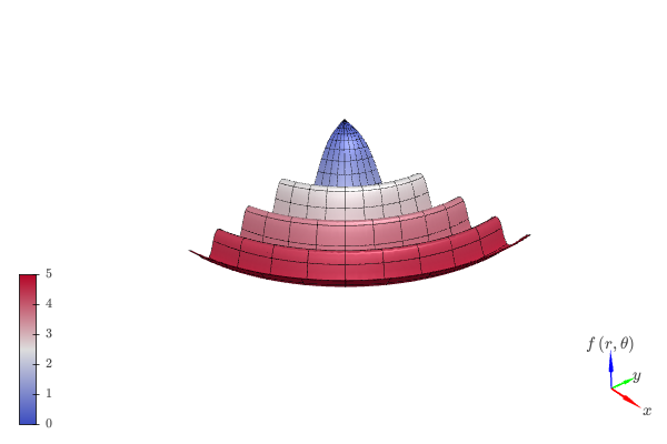
Single plot with a polar discretization, a color function mapping a colormap to the radius. Note that the same result can be achieved with
plot3d_revolution.from sympy import * from spb import * import numpy as np r, theta = symbols("r, theta") expr = cos(r**2) * exp(-r / 3) plot3d(expr, (r, 0, 5), (theta, 1.6 * pi, 2 * pi), backend=KB, is_polar=True, legend=True, grid=False, use_cm=True, color_func=lambda x, y, z: np.sqrt(x**2 + y**2), wireframe=True, wf_n1=30, wf_n2=10, wf_rendering_kw={"width": 0.005})
Plotting a numerical function instead of a symbolic expression:
>>> plot3d(lambda x, y: x * np.exp(-x**2 - y**2),
...     ("x", -3, 3), ("y", -3, 3), use_cm=True)
(
Source code,png,hires.png,pdf)
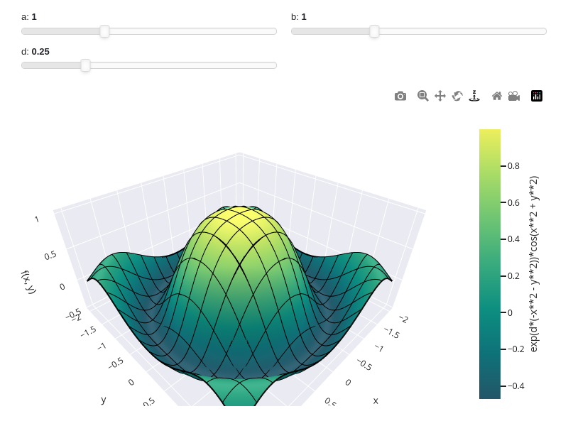
Interactive-widget plot. Refer to the interactive sub-module documentation to learn more about the
paramsdictionary. This plot illustrates:the use of
prange(parametric plotting range).the use of the
paramsdictionary to specify sliders in their basic form: (default, min, max).
from sympy import *
from spb import *
x, y, a, b, d = symbols("x y a b d")
plot3d(
    cos(x**2 + y**2) * exp(-(x**2 + y**2) * d),
    prange(x, -2*a, 2*a), prange(y, -2*b, 2*b),
    params={
        a: (1, 0, 3),
        b: (1, 0, 3),
        d: (0.25, 0, 1),
    },
    backend=PB, use_cm=True, n=100, aspect=dict(x=1.5, y=1.5, z=0.75),
    wireframe=True, wf_n1=15, wf_n2=15, throttled=True, use_latex=False)

- spb.functions.plot3d_parametric_line(*args, **kwargs)[source]
Plots a 3D parametric line plot.
Typical usage examples are in the followings:
- Plotting a single expression.
plot3d_parametric_line(expr_x, expr_y, expr_z, range, **kwargs)
- Plotting a single expression with a custom label and rendering options.
plot3d_parametric_line(expr_x, expr_y, expr_z, range, label, rendering_kw, **kwargs)
- Plotting multiple expressions with the same ranges.
plot3d_parametric_line((expr_x1, expr_y1, expr_z1), (expr_x2, expr_y2, expr_z2), …, range, **kwargs)
- Plotting multiple expressions with different ranges.
plot3d_parametric_line((expr_x1, expr_y1, expr_z1, range1), (expr_x2, expr_y2, expr_z2, range2), …, **kwargs)
- Plotting multiple expressions with custom labels and rendering options.
plot3d_parametric_line((expr_x1, expr_y1, expr_z1, range1, label1, rendering_kw1), (expr_x2, expr_y2, expr_z2, range2, label1, rendering_kw2), …, **kwargs)
- Parameters:
- args
- expr_xExpr
The expression representing x component of the parametric function. It can be a:
Symbolic expression representing the function of one variable to be plotted.
Numerical function of one variable, supporting vectorization. In this case the following keyword arguments are not supported:
params.
- expr_yExpr
The expression representing y component of the parametric function. It can be a:
Symbolic expression representing the function of one variable to be plotted.
Numerical function of one variable, supporting vectorization. In this case the following keyword arguments are not supported:
params.
- expr_zExpr
The expression representing z component of the parametric function. It can be a:
Symbolic expression representing the function of one variable to be plotted.
Numerical function of one variable, supporting vectorization. In this case the following keyword arguments are not supported:
params.
- range(symbol, min, max)
A 3-tuple denoting the range of the parameter variable.
- labelstr, optional
An optional string denoting the label of the expression to be visualized on the legend. If not provided, the string representation of the expression will be used.
- rendering_kwdict, optional
A dictionary of keywords/values which is passed to the backend’s function to customize the appearance of lines. Refer to the plotting library (backend) manual for more informations.
- adaptivebool, optional
Setting
adaptive=Trueactivates the adaptive algorithm implemented in [2] to create smooth plots. Useadaptive_goalandloss_fnto further customize the output.The default value is
False, which uses an uniform sampling strategy, where the number of discretization points is specified by thenkeyword argument.- adaptive_goalcallable, int, float or None
Controls the “smoothness” of the evaluation. Possible values:
None(default): it will use the following goal:lambda l: l.loss() < 0.01number (int or float). The lower the number, the more evaluation points. This number will be used in the following goal:
lambda l: l.loss() < numbercallable: a function requiring one input element, the learner. It must return a float number. Refer to [2] for more information.
- backendPlot, optional
A subclass of
Plot, which will perform the rendering. Default toMatplotlibBackend.- colorbarboolean, optional
Show/hide the colorbar. Default to True (colorbar is visible). Only works when
use_cm=True.- color_funccallable, optional
Define the line color mapping when
use_cm=True. It can either be:A numerical function supporting vectorization. The arity can be:
1 argument:
f(t), wheretis the parameter.3 arguments:
f(x, y, z)wherex, y, zare the coordinates of the points.4 arguments:
f(x, y, z, t).
A symbolic expression having at most as many free symbols as
expr_xorexpr_yorexpr_z.None: the default value (color mapping applied to the parameter).
- force_real_evalboolean, optional
Default to False, with which the numerical evaluation is attempted over a complex domain, which is slower but produces correct results. Set this to True if performance is of paramount importance, but be aware that it might produce wrong results. It only works with
adaptive=False.- is_pointboolean, optional
Default to False, which will render a line connecting all the points. If True, a scatter plot will be generated.
- labelstr or list/tuple, optional
The label to be shown in the legend or in the colorbar. If not provided, the string representation of
exprwill be used. The number of labels must be equal to the number of expressions.- legendbool, optional
Show/hide the legend. Default to None (the backend determines when it is appropriate to show it). Only works when
use_cm=False.- loss_fncallable or None
The loss function to be used by the adaptive learner. Possible values:
None(default): it will use thedefault_lossfrom theadaptivemodule.callable : Refer to [2] for more information. Specifically, look at
adaptive.learner.learner1Dto find more loss functions.
- nint, optional
Used when the
adaptive=False. The function is uniformly sampled atnnumber of points. Default value to 1000. If theadaptive=True, this parameter will be ignored.- paramsdict
A dictionary mapping symbols to parameters. This keyword argument enables the interactive-widgets plot, which doesn’t support the adaptive algorithm (meaning it will use
adaptive=False). Learn more by reading the documentation of the interactive sub-module.- rendering_kwdict or list of dicts, optional
A dictionary of keywords/values which is passed to the backend’s function to customize the appearance of lines. Refer to the plotting library (backend) manual for more informations. If a list of dictionaries is provided, the number of dictionaries must be equal to the number of expressions.
- showbool, optional
The default value is set to
True. Set show toFalseand the function will not display the plot. The returned instance of thePlotclass can then be used to save or display the plot by calling thesave()andshow()methods respectively.- size(float, float), optional
A tuple in the form (width, height) to specify the size of the overall figure. The default value is set to
None, meaning the size will be set by the backend.- titlestr, optional
Title of the plot. It is set to the latex representation of the expression, if the plot has only one expression.
- tx, ty, tz, tpcallable, optional
Apply a numerical function to the x, y, z directions and to the discretized parameter.
- use_cmboolean, optional
If True, apply a color map to the parametric lines. If False, solid colors will be used instead. Default to True.
- use_latexboolean, optional
Turn on/off the rendering of latex labels. If the backend doesn’t support latex, it will render the string representations instead.
- xlabel, ylabel, zlabelstr, optional
Labels for the x-axis, y-axis, z-axis, respectively.
- xlim, ylim, zlim(float, float), optional
Denotes the axis limits, (min, max), visible in the chart.
See also
References
Examples
Note: for documentation purposes, the following examples uses Matplotlib. However, Matplotlib’s 3D capabilities are rather limited. Consider running these examples with a different backend (hence, modify
rendering_kwto pass the correct options to the backend).>>> from sympy import symbols, cos, sin, pi, root >>> from spb import plot3d_parametric_line >>> t = symbols('t')
Single plot.
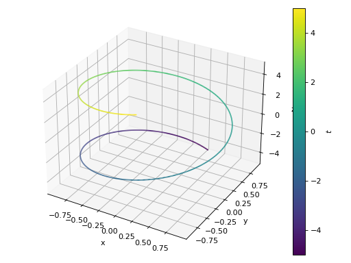
>>> plot3d_parametric_line(cos(t), sin(t), t, (t, -5, 5))
Plot object containing:
[0]: 3D parametric cartesian line: (cos(t), sin(t), t) for t over (-5.0, 5.0)
(
Source code,png,hires.png,pdf)
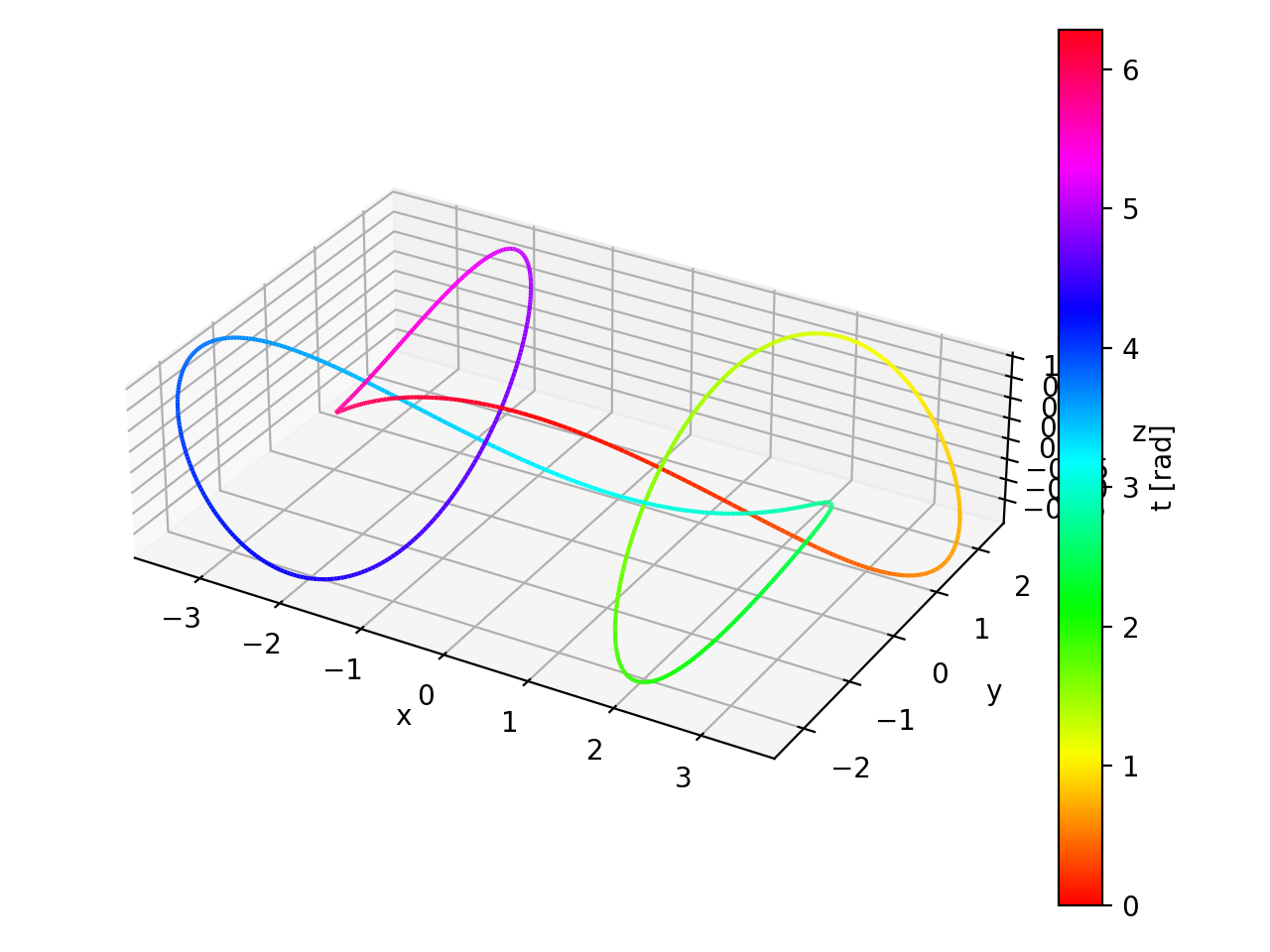
Customize the appearance by setting a label to the colorbar, changing the colormap and the line width.
>>> plot3d_parametric_line(
...     3 * sin(t) + 2 * sin(3 * t), cos(t) - 2 * cos(3 * t), cos(5 * t),
...     (t, 0, 2 * pi), "t [rad]", {"cmap": "hsv", "lw": 1.5},
...     aspect="equal")
Plot object containing:
[0]: 3D parametric cartesian line: (3*sin(t) + 2*sin(3*t), cos(t) - 2*cos(3*t), cos(5*t)) for t over (0.0, 6.283185307179586)
(
Source code,png,hires.png,pdf)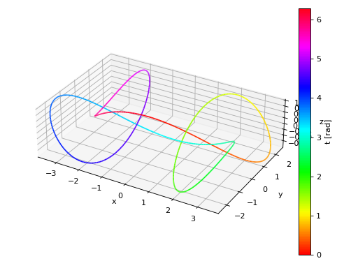
Plot multiple parametric 3D lines with different ranges:
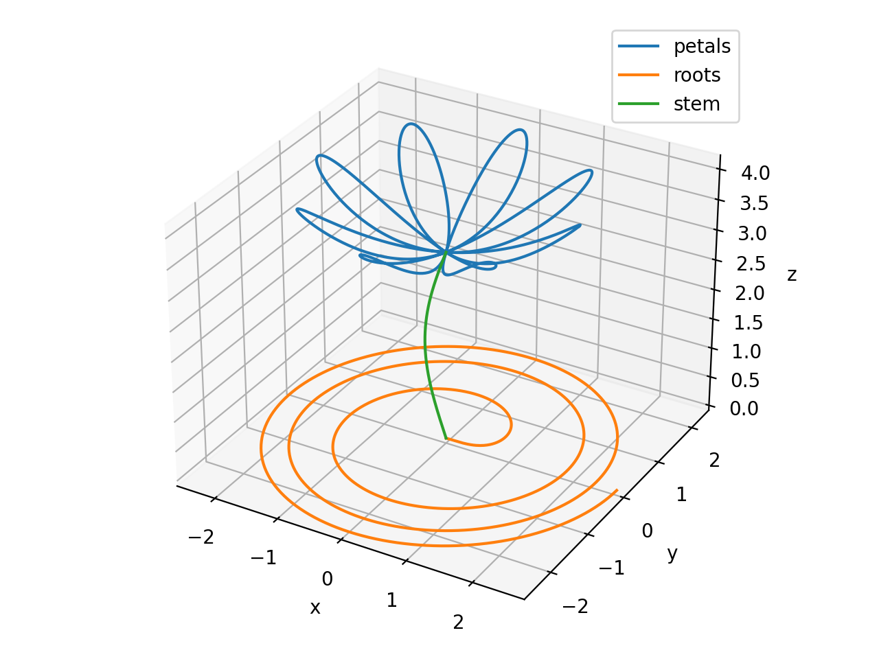
>>> a, b, n = 2, 1, 4
>>> p, r, s = symbols("p r s")
>>> xp = a * cos(p) * cos(n * p)
>>> yp = a * sin(p) * cos(n * p)
>>> zp = b * cos(n * p)**2 + pi
>>> xr = root(r, 3) * cos(r)
>>> yr = root(r, 3) * sin(r)
>>> zr = 0
>>> plot3d_parametric_line(
...     (xp, yp, zp, (p, 0, pi if n % 2 == 1 else 2 * pi), "petals"),
...     (xr, yr, zr, (r, 0, 6*pi), "roots"),
...     (-sin(s)/3, 0, s, (s, 0, pi), "stem"), use_cm=False)
Plot object containing:
[0]: 3D parametric cartesian line: (2*cos(p)*cos(4*p), 2*sin(p)*cos(4*p), cos(4*p)**2 + pi) for p over (0.0, 6.283185307179586)
[1]: 3D parametric cartesian line: (r**(1/3)*cos(r), r**(1/3)*sin(r), 0) for r over (0.0, 18.84955592153876)
[2]: 3D parametric cartesian line: (-sin(s)/3, 0, s) for s over (0.0, 3.141592653589793)
(
Source code,png,hires.png,pdf)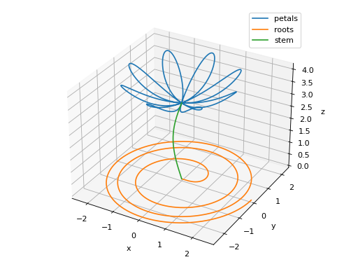
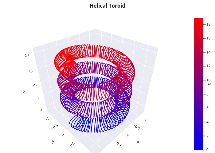
Plotting a numerical function instead of a symbolic expression, using Plotly:
from spb import plot3d_parametric_line, PB
import numpy as np
fx = lambda t: (1 + 0.25 * np.cos(75 * t)) * np.cos(t)
fy = lambda t: (1 + 0.25 * np.cos(75 * t)) * np.sin(t)
fz = lambda t: t + 2 * np.sin(75 * t)
plot3d_parametric_line(fx, fy, fz, ("t", 0, 6 * np.pi),
    {"line": {"colorscale": "bluered"}},
    title="Helical Toroid", backend=PB, adaptive=False, n=1e04)
(Source code, png, pdf, html)
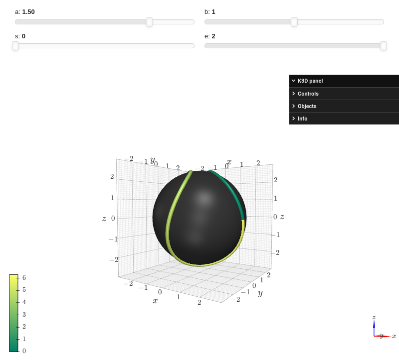
Interactive-widget plot of the parametric line over a tennis ball. Refer to the interactive sub-module documentation to learn more about the
paramsdictionary. This plot illustrates:combining together different plots.
the use of
prange(parametric plotting range).the use of the
paramsdictionary to specify sliders in their basic form: (default, min, max).
from sympy import *
from spb import *
import k3d
a, b, s, e, t = symbols("a, b, s, e, t")
c = 2 * sqrt(a * b)
r = a + b
params = {
    a: (1.5, 0, 2),
    b: (1, 0, 2),
    s: (0, 0, 2),
    e: (2, 0, 2)
}
sphere = plot3d_revolution(
    (r * cos(t), r * sin(t)), (t, 0, pi),
    params=params, n=50, parallel_axis="x",
    backend=KB,
    show_curve=False, show=False,
    rendering_kw={"color":0x353535})
line = plot3d_parametric_line(
    a * cos(t) + b * cos(3 * t),
    a * sin(t) - b * sin(3 * t),
    c * sin(2 * t), prange(t, s*pi, e*pi),
    {"color_map": k3d.matplotlib_color_maps.Summer}, params=params,
    backend=KB, show=False, use_latex=False)
(line + sphere).show()

- spb.functions.plot3d_parametric_surface(*args, **kwargs)[source]
Plots a 3D parametric surface plot.
Typical usage examples are in the followings:
- Plotting a single expression.
plot3d_parametric_surface(expr_x, expr_y, expr_z, range_u, range_v, label, **kwargs)
- Plotting multiple expressions with the same ranges.
plot3d_parametric_surface((expr_x1, expr_y1, expr_z1), (expr_x2, expr_y2, expr_z2), range_u, range_v, **kwargs)
- Plotting multiple expressions with different ranges.
plot3d_parametric_surface((expr_x1, expr_y1, expr_z1, range_u1, range_v1), (expr_x2, expr_y2, expr_z2, range_u2, range_v2), **kwargs)
- Plotting multiple expressions with different ranges and rendering option.
plot3d_parametric_surface((expr_x1, expr_y1, expr_z1, range_u1, range_v1, label1, rendering_kw1), (expr_x2, expr_y2, expr_z2, range_u2, range_v2, label2, rendering_kw2), **kwargs)
Note: it is important to specify both the ranges.
- Parameters:
- args
- expr_x: Expr
Expression representing the function along x. It can be a:
Symbolic expression.
Numerical function of two variable, f(u, v), supporting vectorization. In this case the following keyword arguments are not supported:
params.
- expr_y: Expr
Expression representing the function along y. It can be a:
Symbolic expression.
Numerical function of two variable, f(u, v), supporting vectorization. In this case the following keyword arguments are not supported:
params.
- expr_z: Expr
Expression representing the function along z. It can be a:
Symbolic expression.
Numerical function of two variable, f(u, v), supporting vectorization. In this case the following keyword arguments are not supported:
params.
- range_u: (symbol, min, max)
A 3-tuple denoting the range of the u variable.
- range_v: (symbol, min, max)
A 3-tuple denoting the range of the v variable.
- labelstr, optional
The label to be shown in the colorbar. If not provided, the string representation of the expression will be used.
- rendering_kwdict, optional
A dictionary of keywords/values which is passed to the backend’s function to customize the appearance of surfaces. Refer to the plotting library (backend) manual for more informations.
- backendPlot, optional
A subclass of
Plot, which will perform the rendering. Default toMatplotlibBackend.- colorbarboolean, optional
Show/hide the colorbar. Default to True (colorbar is visible). Only works when
use_cm=True.- color_funccallable, optional
Define the surface color mapping when
use_cm=True. It can either be:A numerical function supporting vectorization. The arity can be:
1 argument:
f(u), whereuis the first parameter.2 arguments:
f(u, v)whereu, vare the parameters.3 arguments:
f(x, y, z)wherex, y, zare the coordinates of the points.5 arguments:
f(x, y, z, u, v).
A symbolic expression having at most as many free symbols as
expr_xorexpr_yorexpr_z.None: the default value (color mapping applied to the z-value of the surface).
- force_real_evalboolean, optional
Default to False, with which the numerical evaluation is attempted over a complex domain, which is slower but produces correct results. Set this to True if performance is of paramount importance, but be aware that it might produce wrong results. It only works with
adaptive=False.- labelstr or list/tuple, optional
The label to be shown in the colorbar. If not provided, the string representation will be used. The number of labels must be equal to the number of expressions.
- n1, n2int, optional
n1andn2set the number of discretization points along the u and v ranges, respectively. Default value to 100.- nint or two-elements tuple (n1, n2), optional
If an integer is provided, the u and v ranges are sampled uniformly at
nof points. If a tuple is provided, it overridesn1andn2.- legendbool, optional
Show/hide the legend. Default to None (the backend determines when it is appropriate to show it). Only works when
use_cm=False.- paramsdict
A dictionary mapping symbols to parameters. This keyword argument enables the interactive-widgets plot. Learn more by reading the documentation of the interactive sub-module.
- rendering_kwdict or list of dicts, optional
A dictionary of keywords/values which is passed to the backend’s function to customize the appearance of surfaces. Refer to the plotting library (backend) manual for more informations. If a list of dictionaries is provided, the number of dictionaries must be equal to the number of expressions.
- showbool, optional
The default value is set to
True. Set show toFalseand the function will not display the plot. The returned instance of thePlotclass can then be used to save or display the plot by calling thesave()andshow()methods respectively.- size(float, float), optional
A tuple in the form (width, height) to specify the size of the overall figure. The default value is set to
None, meaning the size will be set by the backend.- titlestr, optional
Title of the plot. It is set to the latex representation of the expression, if the plot has only one expression.
- tx, ty, tzcallable, optional
Apply a numerical function to the discretized domain in the x, y and z direction, respectively.
- use_cmboolean, optional
If True, apply a color map to the surface. If False, solid colors will be used instead. Default to False.
- use_latexboolean, optional
Turn on/off the rendering of latex labels. If the backend doesn’t support latex, it will render the string representations instead.
- wireframeboolean, optional
Enable or disable a wireframe over the surface. Depending on the number of wireframe lines (see
wf_n1andwf_n2), activating this option might add a considerable overhead during the plot’s creation. Default to False (disabled).- wf_n1, wf_n2int, optional
Number of wireframe lines along the u and v ranges, respectively. Default to 10. Note that increasing this number might considerably slow down the plot’s creation.
- wf_npointint or None, optional
Number of discretization points for the wireframe lines. Default to None, meaning that each wireframe line will have
n1orn2number of points, depending on the line direction.- wf_rendering_kwdict, optional
A dictionary of keywords/values which is passed to the backend’s function to customize the appearance of wireframe lines.
- xlabel, ylabel, zlabelstr, optional
Label for the x-axis or y-axis or z-axis, respectively.
- xlim, ylim, zlim(float, float), optional
Denotes the x-axis limits, or y-axis limits, or z-axis limits, respectively,
(min, max), visible in the chart.
See also
plot3d,plot3d_parametric_list,plot3d_sphericalplot3d_revolution,plot3d_implicit,plot3d_list
Examples
Note: for documentation purposes, the following examples uses Matplotlib. However, Matplotlib’s 3D capabilities are rather limited. Consider running these examples with a different backend (hence, modify the
rendering_kwandwf_rendering_kwto pass the correct options to the backend).>>> from sympy import symbols, cos, sin, pi, I, sqrt, atan2, re, im >>> from spb import plot3d_parametric_surface >>> u, v = symbols('u v')
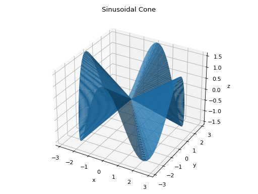
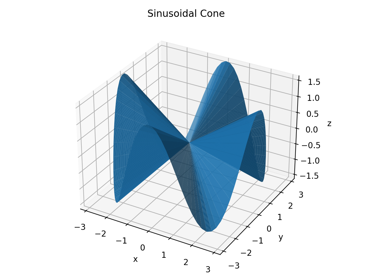
Plot a parametric surface:
>>> plot3d_parametric_surface(
...     u * cos(v), u * sin(v), u * cos(4 * v) / 2,
...     (u, 0, pi), (v, 0, 2*pi),
...     use_cm=False, title="Sinusoidal Cone")
Plot object containing:
[0]: parametric cartesian surface: (u*cos(v), u*sin(v), u*cos(4*v)/2) for u over (0.0, 3.141592653589793) and v over (0.0, 6.283185307179586)
(
Source code,png,hires.png,pdf)
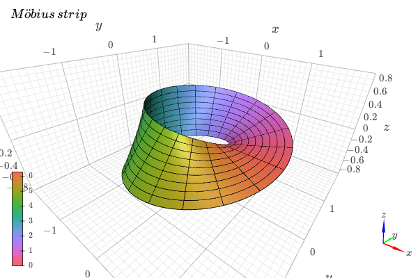
Customize the appearance of the surface by changing the colormap. Apply a color function mapping the v values. Activate the wireframe to better visualize the parameterization.
from sympy import *
from spb import *
import k3d
var("u, v")

x = (1 + v / 2 * cos(u / 2)) * cos(u)
y = (1 + v / 2 * cos(u / 2)) * sin(u)
z = v / 2 * sin(u / 2)
plot3d_parametric_surface(
    x, y, z, (u, 0, 2*pi), (v, -1, 1),
    "v", {"color_map": k3d.colormaps.paraview_color_maps.Hue_L60},
    backend=KB,
    use_cm=True, color_func=lambda u, v: u,
    title="Möbius \, strip",
    wireframe=True, wf_n1=20, wf_rendering_kw={"width": 0.004})
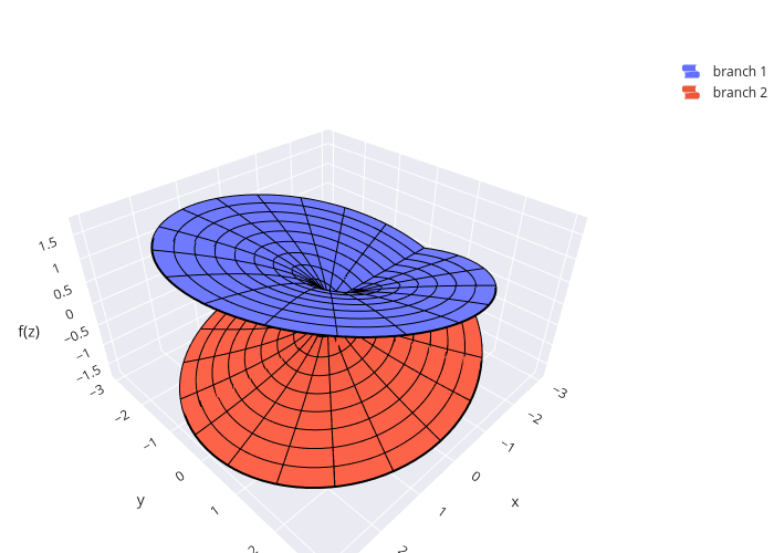
Riemann surfaces of the real part of the multivalued function z**n, using Plotly:
from sympy import symbols, sqrt, re, im, pi, atan2, sin, cos, I
from spb import plot3d_parametric_surface, PB
r, theta, x, y = symbols("r, theta, x, y", real=True)
mag = lambda z: sqrt(re(z)**2 + im(z)**2)
phase = lambda z, k=0: atan2(im(z), re(z)) + 2 * k * pi
n = 2 # exponent (integer)
z = x + I * y # cartesian
d = {x: r * cos(theta), y: r * sin(theta)} # cartesian to polar
branches = [(mag(z)**(1 / n) * cos(phase(z, i) / n)).subs(d)
    for i in range(n)]
exprs = [(r * cos(theta), r * sin(theta), rb) for rb in branches]
plot3d_parametric_surface(*exprs, (r, 0, 3), (theta, -pi, pi),
    backend=PB, wireframe=True, wf_n2=20, zlabel="f(z)",
    label=["branch %s" % (i + 1) for i in range(len(branches))])
(Source code, png, pdf, html)
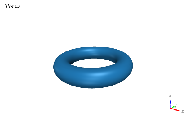
Plotting a numerical function instead of a symbolic expression.
from spb import *
import numpy as np
fx = lambda u, v: (4 + np.cos(u)) * np.cos(v)
fy = lambda u, v: (4 + np.cos(u)) * np.sin(v)
fz = lambda u, v: np.sin(u)
plot3d_parametric_surface(fx, fy, fz, ("u", 0, 2 * np.pi),
    ("v", 0, 2 * np.pi), zlim=(-2.5, 2.5), title="Torus",
    backend=KB, grid=False)

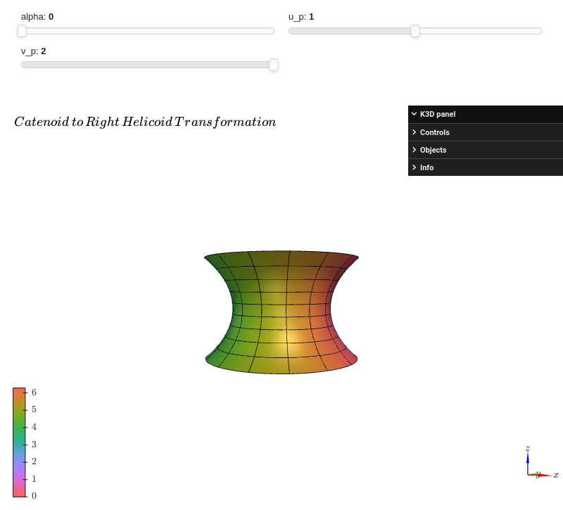
Interactive-widget plot. Refer to the interactive sub-module documentation to learn more about the
paramsdictionary. This plot illustrates:the use of
prange(parametric plotting range).the use of the
paramsdictionary to specify sliders in their basic form: (default, min, max).
from sympy import *
from spb import *
import k3d
alpha, u, v, up, vp = symbols("alpha u v u_p v_p")
plot3d_parametric_surface((
        exp(u) * cos(v - alpha) / 2 + exp(-u) * cos(v + alpha) / 2,
        exp(u) * sin(v - alpha) / 2 + exp(-u) * sin(v + alpha) / 2,
        cos(alpha) * u + sin(alpha) * v
    ),
    prange(u, -up, up), prange(v, 0, vp * pi),
    backend=KB,
    use_cm=True,
    color_func=lambda u, v: v,
    rendering_kw={"color_map": k3d.colormaps.paraview_color_maps.Hue_L60},
    wireframe=True, wf_n2=15, wf_rendering_kw={"width": 0.005},
    grid=False, n=50, use_latex=False,
    params={
        alpha: (0, 0, pi),
        up: (1, 0, 2),
        vp: (2, 0, 2),
    },
    title="Catenoid \, to \, Right \, Helicoid \, Transformation")

Interactive-widget plot. Refer to the interactive sub-module documentation to learn more about the
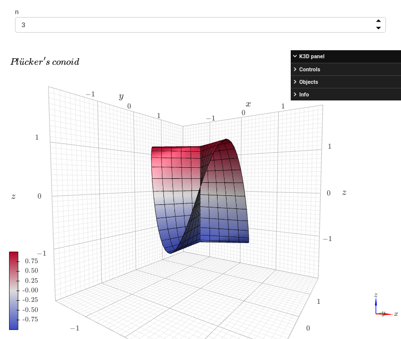
paramsdictionary. Note that the plot’s creation might be slow due to the wireframe lines.from sympy import * from spb import * import param n, u, v = symbols("n, u, v") x = v * cos(u) y = v * sin(u) z = sin(n * u) plot3d_parametric_surface( (x, y, z, (u, 0, 2*pi), (v, -1, 0)), params = { n: param.Integer(3, label="n") }, backend=KB, use_cm=True, title=r"Plücker's \, conoid", wireframe=True, wf_rendering_kw={"width": 0.004}, wf_n1=75, wf_n2=6, imodule="panel" )

- spb.functions.plot3d_spherical(*args, **kwargs)[source]
Plots a radius as a function of the spherical coordinates theta and phi.
Typical usage examples are in the followings:
- Plotting a single expression.
plot3d_spherical(r, range_theta, range_phi, **kwargs)
- Plotting multiple expressions with the same ranges.
plot3d_parametric_surface(r1, r2, range_theta, range_phi, **kwargs)
- Plotting multiple expressions with different ranges.
plot3d_parametric_surface((r1, range_theta1, range_phi1), (r2, range_theta2, range_phi2), **kwargs)
- Plotting multiple expressions with different ranges and rendering option.
plot3d_parametric_surface((r1, range_theta1, range_phi1, label1, rendering_kw1), (r2, range_theta2, range_phi2, label2, rendering_kw2), **kwargs)
Note: it is important to specify both the ranges.
- Parameters:
- args
- r: Expr
Expression representing the radius. It can be a:
Symbolic expression.
Numerical function of two variable, f(theta, phi), supporting vectorization. In this case the following keyword arguments are not supported:
params.
- theta: (symbol, min, max)
A 3-tuple denoting the range of the polar angle, which is limited in [0, pi]. Consider a sphere:
theta=0indicates the north pole.theta=pi/2indicates the equator.theta=piindicates the south pole.
- range_v: (symbol, min, max)
A 3-tuple denoting the range of the azimuthal angle, which is limited in [0, 2*pi].
- labelstr, optional
The label to be shown in the colorbar. If not provided, the string representation of the expression will be used.
- rendering_kwdict, optional
A dictionary of keywords/values which is passed to the backend’s function to customize the appearance of surfaces. Refer to the plotting library (backend) manual for more informations.
**kwargs:Keyword arguments are the same as
plot3d_parametric_surface. Refer to its documentation for more information.
See also
plot3d,plot3d_parametric_list,plot3d_parametric_surfaceplot3d_revolution,plot3d_implicit,plot3d_list
Examples
Note: for documentation purposes, the following examples uses Matplotlib. However, Matplotlib’s 3D capabilities are rather limited. Consider running these examples with a different backend (hence, modify the
rendering_kwandwf_rendering_kwto pass the correct options to the backend).>>> from sympy import symbols, cos, sin, pi, Ynm, re, lambdify >>> from spb import plot3d_spherical >>> theta, phi = symbols('theta phi')
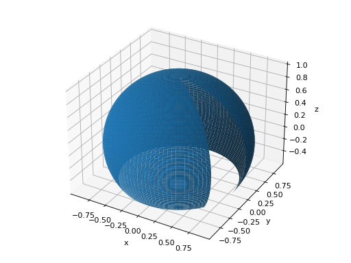
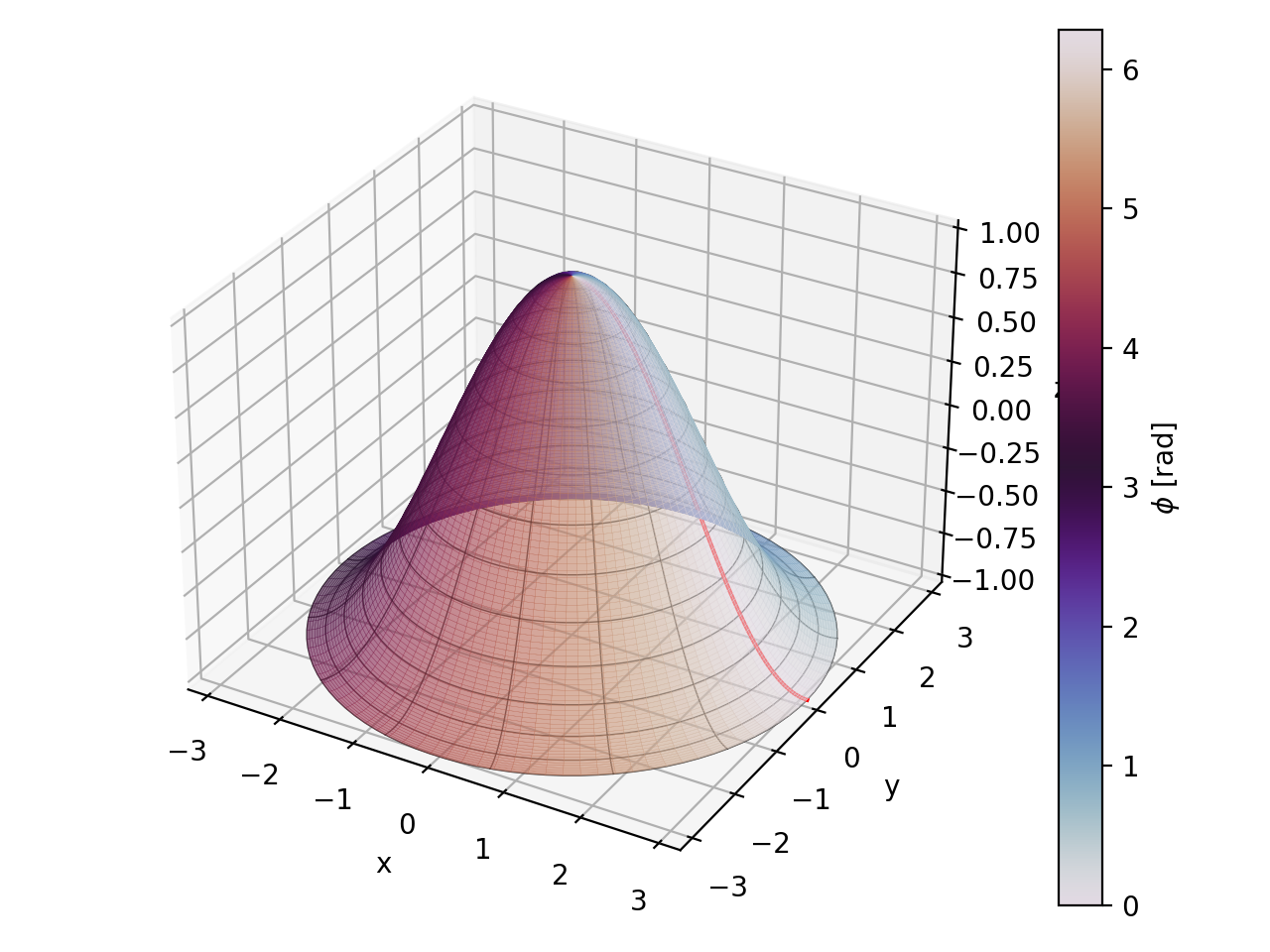
Sphere cap:
>>> plot3d_spherical(1, (theta, 0, 0.7 * pi), (phi, 0, 1.8 * pi))
Plot object containing:
[0]: parametric cartesian surface: (sin(theta)*cos(phi), sin(phi)*sin(theta), cos(theta)) for theta over (0.0, 2.199114857512855) and phi over (0.0, 5.654866776461628)
(
Source code,png,hires.png,pdf)
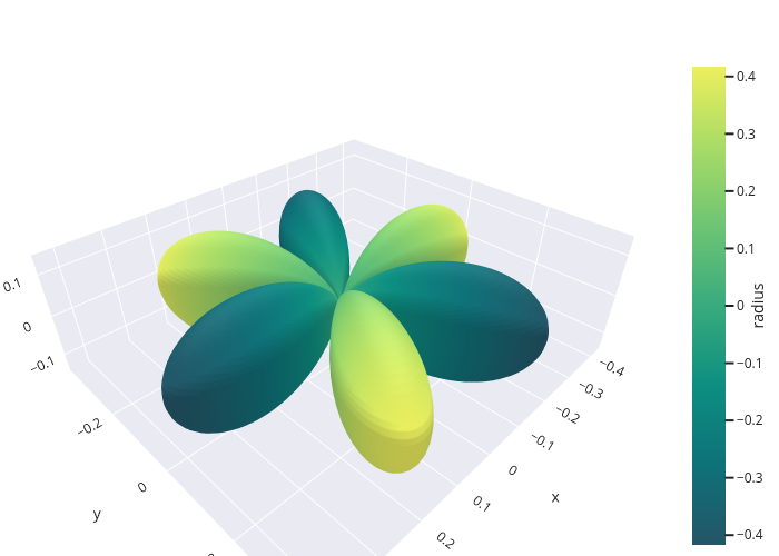
Plot real spherical harmonics, highlighting the regions in which the real part is positive and negative, using Plotly:
from sympy import symbols, sin, pi, Ynm, re, lambdify
from spb import plot3d_spherical, PB
theta, phi = symbols('theta phi')
r = re(Ynm(3, 3, theta, phi).expand(func=True).rewrite(sin).expand())
plot3d_spherical(
    abs(r), (theta, 0, pi), (phi, 0, 2 * pi), "radius",
    use_cm=True, n2=200, backend=PB,
    color_func=lambdify([theta, phi], r))
(Source code, png, pdf, html)
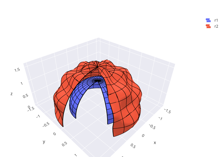
Multiple surfaces with wireframe lines, using Plotly. Note that activating the wireframe option might add a considerable overhead during the plot’s creation.
from sympy import symbols, sin, pi
from spb import plot3d_spherical, PB
theta, phi = symbols('theta phi')
r1 = 1
r2 = 1.5 + sin(5 * phi) * sin(10 * theta) / 10
plot3d_spherical(r1, r2, (theta, 0, pi / 2), (phi, 0.35 * pi, 2 * pi),
    wireframe=True, wf_n2=25, backend=PB, label=["r1", "r2"])
(Source code, png, pdf, html)
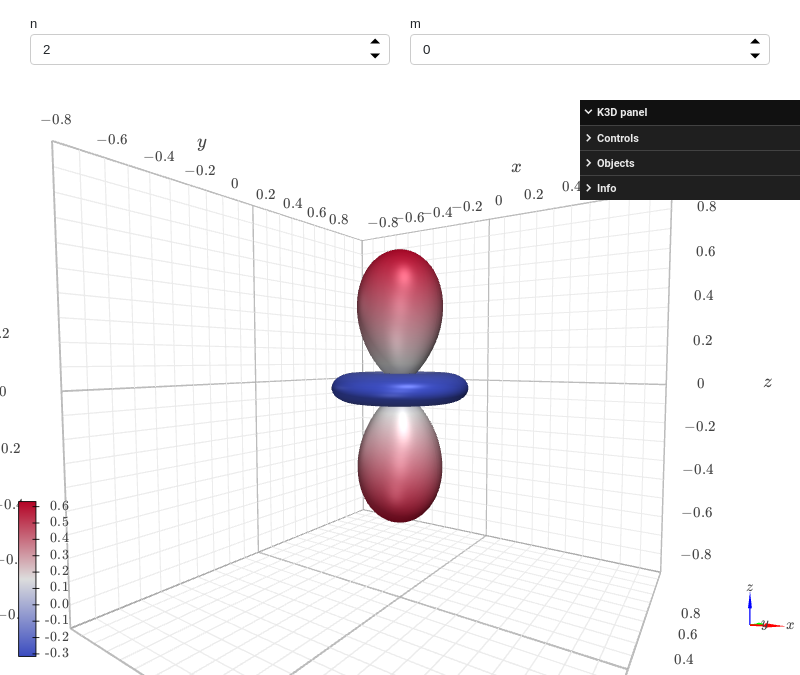
Interactive-widget plot of real spherical harmonics, highlighting the regions in which the real part is positive and negative. Note that the plot’s creation and update might be slow and that it must be
m < nat all times. Refer to the interactive sub-module documentation to learn more about theparamsdictionary.from sympy import * from spb import * import param n, m = symbols("n, m") phi, theta = symbols("phi, theta", real=True) r = re(Ynm(n, m, theta, phi).expand(func=True).rewrite(sin).expand()) plot3d_spherical( abs(r), (theta, 0, pi), (phi, 0, 2*pi), params = { n: param.Integer(2, label="n"), m: param.Integer(0, label="m"), }, force_real_eval=True, use_cm=True, color_func=r, backend=KB, imodule="panel")

- spb.functions.plot3d_revolution(curve, range_t, range_phi=None, axis=(0, 0), parallel_axis='z', show_curve=False, curve_kw=None, **kwargs)[source]
Generate a surface of revolution by rotating a curve around an axis of rotation.
- Parameters:
- curveExpr, list/tuple of 2 or 3 elements
The curve to be revolved, which can be either:
a symbolic expression
a 2-tuple representing a parametric curve in 2D space
a 3-tuple representing a parametric curve in 3D space
- range_t(symbol, min, max)
A 3-tuple denoting the range of the parameter of the curve.
- range_phi(symbol, min, max)
A 3-tuple denoting the range of the azimuthal angle where the curve will be revolved. Default to
(phi, 0, 2*pi).- axis(coord1, coord2)
A 2-tuple that specifies the position of the rotation axis. Depending on the value of
parallel_axis:"x": the rotation axis intersects the YZ plane at (coord1, coord2)."y": the rotation axis intersects the XZ plane at (coord1, coord2)."z": the rotation axis intersects the XY plane at (coord1, coord2).
Default to
(0, 0).- parallel_axisstr
Specify the axis parallel to the axis of rotation. Must be one of the following options: “x”, “y” or “z”. Default to “z”.
- show_curvebool
Add the initial curve to the plot. Default to False.
- curve_kwdict
A dictionary of options that will be passed to
plot3d_parametric_lineifshow_curve=Truein order to customize the appearance of the initial curve. Refer to its documentation for more information.- ``**kwargs``
Keyword arguments are the same as
plot3d_parametric_surface. Refer to its documentation for more information.
See also
plot3d,plot3d_parametric_list,plot3d_parametric_surfaceplot3d_spherical,plot3d_implicit,plot3d_list
Examples
Note: for documentation purposes, the following examples uses Matplotlib. However, Matplotlib’s 3D capabilities are rather limited. Consider running these examples with a different backend (hence, modify the
curve_kw,rendering_kwandwf_rendering_kwto pass the correct options to the backend).>>> from sympy import symbols, cos, sin, pi >>> from spb import plot3d_revolution >>> t, phi = symbols('t phi')
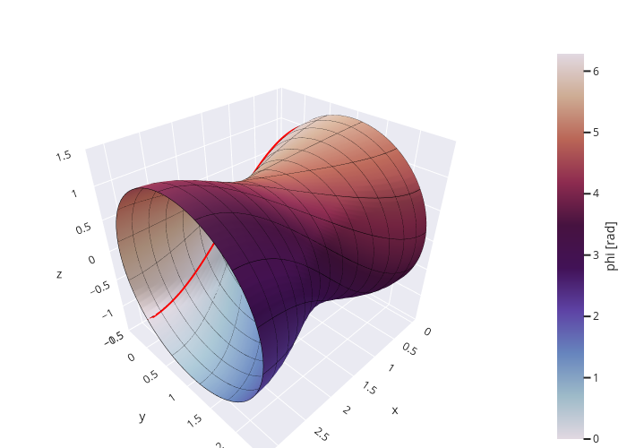
Revolve a function around the z axis:
>>> plot3d_revolution(
...     cos(t), (t, 0, pi),
...     # use a color map on the surface to indicate the azimuthal angle
...     use_cm=True, color_func=lambda t, phi: phi,
...     rendering_kw={"alpha": 0.6, "cmap": "twilight"},
...     # indicates the azimuthal angle on the colorbar label
...     label=r"$\phi$ [rad]",
...     show_curve=True,
...     # this dictionary will be passes to plot3d_parametric_line in
...     # order to draw the initial curve
...     curve_kw=dict(rendering_kw={"color": "r", "label": "cos(t)"}),
...     # activate the wireframe to visualize the parameterization
...     wireframe=True, wf_n1=15, wf_n2=15,
...     wf_rendering_kw={"lw": 0.5, "alpha": 0.75})
(
Source code,png,hires.png,pdf)
Revolve the same function around an axis parallel to the x axis, using Plotly:
from sympy import symbols, cos, sin, pi
from spb import plot3d_revolution, PB
t, phi = symbols('t phi')
plot3d_revolution(
    cos(t), (t, 0, pi), parallel_axis="x", axis=(1, 0),
    backend=PB, use_cm=True, color_func=lambda t, phi: phi,
    rendering_kw={"colorscale": "twilight"},
    label="phi [rad]",
    show_curve=True,
    curve_kw=dict(rendering_kw={"line": {"color": "red", "width": 8},
        "name": "cos(t)"}),
    wireframe=True, wf_n1=15, wf_n2=15,
    wf_rendering_kw={"line_width": 1})
(Source code, png, pdf, html)
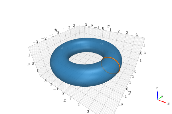
Revolve a 2D parametric circle around the z axis:
from sympy import *
from spb import *
t = symbols("t")
circle = (3 + cos(t), sin(t))
plot3d_revolution(circle, (t, 0, 2 * pi),
    backend=KB, show_curve=True,
    rendering_kw={"opacity": 0.65},
    curve_kw={"rendering_kw": {"width": 0.05}})

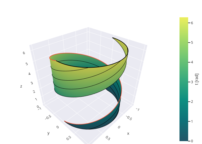
Revolve a 3D parametric curve around the z axis for a given azimuthal angle, using Plotly:
plot3d_revolution(
    (cos(t), sin(t), t), (t, 0, 2*pi), (phi, 0, pi),
    use_cm=True, color_func=lambda t, phi: t, label="t [rad]",
    show_curve=True, backend=PB, aspect="cube",
    wireframe=True, wf_n1=2, wf_n2=5)
(Source code, png, pdf, html)
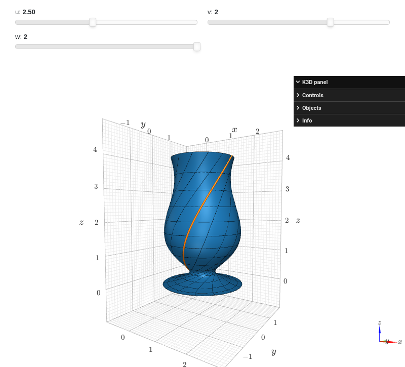
Interactive-widget plot of a goblet. Refer to the interactive sub-module documentation to learn more about the
paramsdictionary. This plot illustrates:the use of
prange(parametric plotting range).the use of the
paramsdictionary to specify sliders in their basic form: (default, min, max).
from sympy import *
from spb import *
t, phi, u, v, w = symbols("t phi u v w")
plot3d_revolution(
    (t, cos(u * t), t**2), prange(t, 0, v), prange(phi, 0, w*pi),
    axis=(1, 0.2),
    params={
        u: (2.5, 0, 6),
        v: (2, 0, 3),
        w: (2, 0, 2)
    }, n=50, backend=KB, force_real_eval=True,
    wireframe=True, wf_n1=15, wf_n2=15,
    wf_rendering_kw={"width": 0.004},
    show_curve=True, curve_kw={"rendering_kw": {"width": 0.025}},
    use_latex=False)
- spb.functions.plot3d_implicit(*args, **kwargs)[source]
Plots an isosurface of a function.
Typical usage examples are in the followings:
plot3d_parametric_surface(expr, range_x, range_y, range_z, rendering_kw [optional], **kwargs)
Note that:
it is important to specify the ranges, as they will determine the orientation of the surface.
the number of discretization points is crucial as the algorithm will discretize a volume. A high number of discretization points creates a smoother mesh, at the cost of a much higher memory consumption and slower computation.
To plot
f(x, y, z) = ceither writeexpr = f(x, y, z) - cor pass the appropriate keyword torendering_kw. Read the backends documentation to find out the available options.Only
PlotlyBackendandK3DBackendsupport 3D implicit plotting.
- Parameters:
- args
- expr: Expr
Implicit expression. It can be a:
Symbolic expression.
Numerical function of three variable, f(x, y, z), supporting vectorization.
- range_x: (symbol, min, max)
A 3-tuple denoting the range of the x variable.
- range_y: (symbol, min, max)
A 3-tuple denoting the range of the y variable.
- range_z: (symbol, min, max)
A 3-tuple denoting the range of the z variable.
- rendering_kwdict, optional
A dictionary of keywords/values which is passed to the backend’s function to customize the appearance of surfaces. Refer to the plotting library (backend) manual for more informations.
- backendPlot, optional
A subclass of
Plot, which will perform the rendering.- n1, n2, n3int, optional
Set the number of discretization points along the x, y and z ranges, respectively. Default value is 60.
- nint or three-elements tuple (n1, n2, n3), optional
If an integer is provided, the x, y and z ranges are sampled uniformly at
nof points. If a tuple is provided, it overridesn1,n2andn3.- rendering_kwdict or list of dicts, optional
A dictionary of keywords/values which is passed to the backend’s function to customize the appearance of surfaces. Refer to the plotting library (backend) manual for more informations. If a list of dictionaries is provided, the number of dictionaries must be equal to the number of expressions.
- showbool, optional
The default value is set to
True. Set show toFalseand the function will not display the plot. The returned instance of thePlotclass can then be used to save or display the plot by calling thesave()andshow()methods respectively.- size(float, float), optional
A tuple in the form (width, height) to specify the size of the overall figure. The default value is set to None, meaning the size will be set by the backend.
- titlestr, optional
Title of the plot. It is set to the latex representation of the expression, if the plot has only one expression.
- use_latexboolean, optional
Turn on/off the rendering of latex labels. If the backend doesn’t support latex, it will render the string representations instead.
- xlabel, ylabel, zlabelstr, optional
Labels for the x-axis, y-axis or z-axis, respectively.
- xlim, ylim, zlim(float, float), optional
Denotes the x-axis limits, y-axis limits or z-axis limits, respectively,
(min, max), visible in the chart. Note that the function is still being evaluated over therange_x,range_yandrange_z.
See also
plot3d,plot3d_parametric_list,plot3d_parametric_surfaceplot3d_spherical,plot3d_revolution,plot3d_list
Examples
from sympy import symbols
from spb import plot3d_implicit, PB, KB
x, y, z = symbols('x, y, z')
plot3d_implicit(
    x**2 + y**3 - z**2, (x, -2, 2), (y, -2, 2), (z, -2, 2), backend=PB)
(Source code, png, pdf, html)
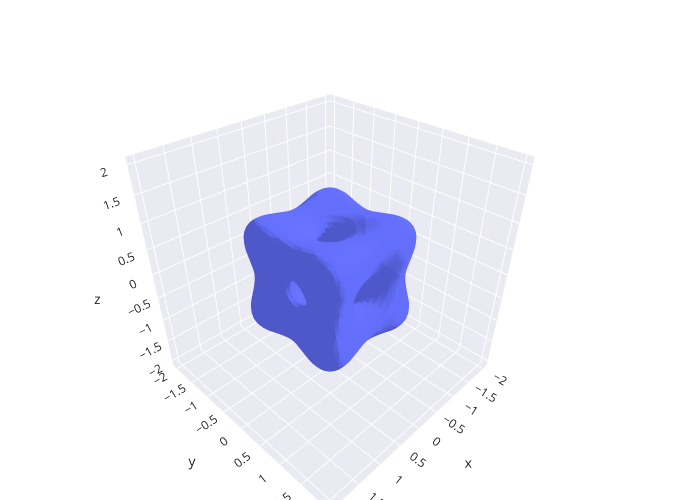
plot3d_implicit(
    x**4 + y**4 + z**4 - (x**2 + y**2 + z**2 - 0.3),
    (x, -2, 2), (y, -2, 2), (z, -2, 2), backend=PB)
(Source code, png, pdf, html)
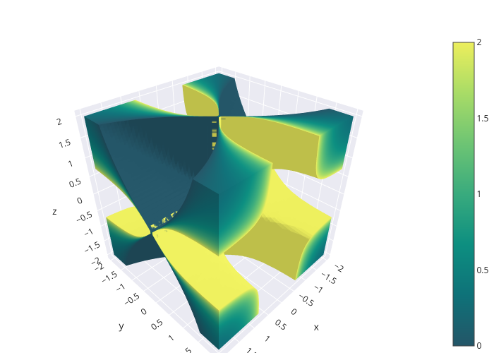
Visualize the isocontours from isomin=0 to isomax=2 by providing a
rendering_kwdictionary:plot3d_implicit( 1/x**2 - 1/y**2 + 1/z**2, (x, -2, 2), (y, -2, 2), (z, -2, 2), { "isomin": 0, "isomax": 2, "colorscale":"aggrnyl", "showscale":True }, backend=PB )
(Source code, png, pdf, html)
- spb.functions.plot3d_list(*args, **kwargs)[source]
Plots lists of coordinates (ie, lists of numbers) in 3D space.
Typical usage examples are in the followings:
- Plotting coordinates of a single function.
plot3d_list(x, y, **kwargs)
- Plotting coordinates of multiple functions adding custom labels.
plot3d_list((x1, y1, label1), (x2, y2, label2), **kwargs)
- Parameters:
- args
- xlist or tuple or 1D NumPy array
x-coordinates
- ylist or tuple or 1D NumPy array
y-coordinates
- zlist or tuple or 1D NumPy array
z-coordinates
- labelstr, optional
The label to be shown in the legend.
- rendering_kwdict, optional
A dictionary of keywords/values which is passed to the backend’s function to customize the appearance of lines. Refer to the plotting library (backend) manual for more informations.
- backendPlot, optional
A subclass of Plot, which will perform the rendering. Default to MatplotlibBackend.
- color_funccallable, optional
A numerical function of 3 variables, x, y, z defining the line color. Default to None. Requires
use_cm=Truein order to be applied.- is_pointboolean, optional
Default to False, which will render a line connecting all the points. If True, a scatter plot will be generated.
- is_filledboolean, optional
Default to True, which will render filled circular markers. It only works if is_point=True. If True, filled circular markers will be rendered. Note that some backend might not support this feature.
- labelstr or list/tuple, optional
The label to be shown in the legend. The number of labels must be equal to the number of expressions.
- legendbool, optional
Show/hide the legend. Default to None (the backend determines when it is appropriate to show it).
- paramsdict
A dictionary mapping symbols to parameters. This keyword argument enables the interactive-widgets plot. Learn more by reading the documentation of the interactive sub-module.
- rendering_kwdict or list of dicts, optional
A dictionary of keywords/values which is passed to the backend’s function to customize the appearance of lines. Refer to the plotting library (backend) manual for more informations. If a list of dictionaries is provided, the number of dictionaries must be equal to the number of expressions.
- showbool, optional
The default value is set to
True. Set show toFalseand the function will not display the plot. The returned instance of thePlotclass can then be used to save or display the plot by calling thesave()andshow()methods respectively.- size(float, float), optional
A tuple in the form (width, height) to specify the size of the overall figure. The default value is set to None, meaning the size will be set by the backend.
- titlestr, optional
Title of the plot. It is set to the latex representation of the expression, if the plot has only one expression.
- use_cmboolean, optional
If True, apply a color map to the parametric lines. If False, solid colors will be used instead. Default to True.
- use_latexboolean, optional
Turn on/off the rendering of latex labels. If the backend doesn’t support latex, it will render the string representations instead.
- xlabel, ylabel, zlabelstr, optional
Label for the x-axis, y-axis, z-axis, respectively.
- xlim, ylim, zlim(float, float), optional
Denotes the x-axis limits, y-axis limits or z-axis limits, respectively,
(min, max), visible in the chart.
See also
plot3d,plot3d_parametric_list,plot3d_parametric_surfaceplot3d_spherical,plot3d_revolution,plot3d_implicit
Examples
>>> from sympy import *
>>> from spb import plot3d_list
>>> import numpy as np
Plot the coordinates of a single function:
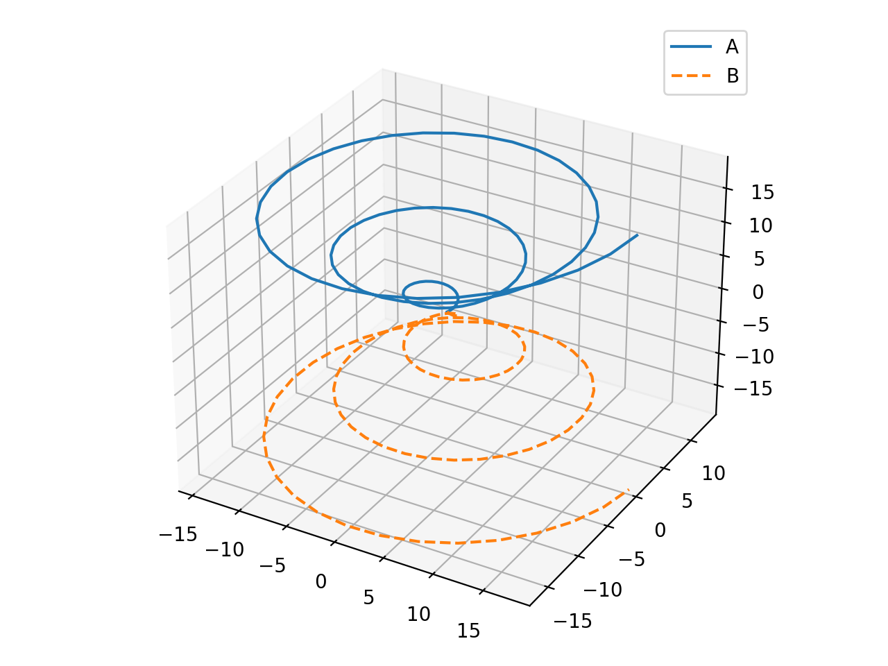
>>> z = np.linspace(0, 6*np.pi, 100)
>>> x = z * np.cos(z)
>>> y = z * np.sin(z)
>>> plot3d_list(x, y, z)
Plot object containing:
[0]: 3D list plot
(
Source code,png,hires.png,pdf)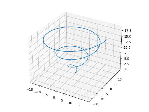
Plotting multiple functions with custom rendering keywords:
>>> plot3d_list(
...     (x, y, z, "A"),
...     (x, y, -z, "B", {"linestyle": "--"}))
Plot object containing:
[0]: 3D list plot
[1]: 3D list plot
(
Source code,png,hires.png,pdf)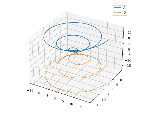
Interactive-widget plot of a dot following a path. Refer to the interactive sub-module documentation to learn more about the
paramsdictionary.from sympy import * from spb import * import numpy as np t = symbols("t") z = np.linspace(0, 6*np.pi, 100) x = z * np.cos(z) y = z * np.sin(z) p1 = plot3d_list(x, y, z, show=False, is_point=False) p2 = plot3d_list( [t * cos(t)], [t * sin(t)], [t], params={t: (3*pi, 0, 6*pi)}, backend=PB, show=False, is_point=True, use_latex=False, imodule="panel") (p2 + p1).show()
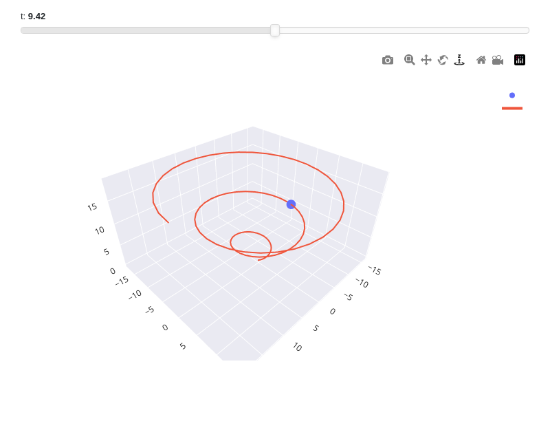