Control
This module contains plotting functions for some of the common plots used in control system.
- spb.control.plot_pole_zero(*systems, pole_markersize=10, zero_markersize=7, show_axes=False, **kwargs)[source]
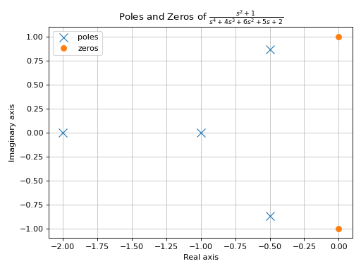
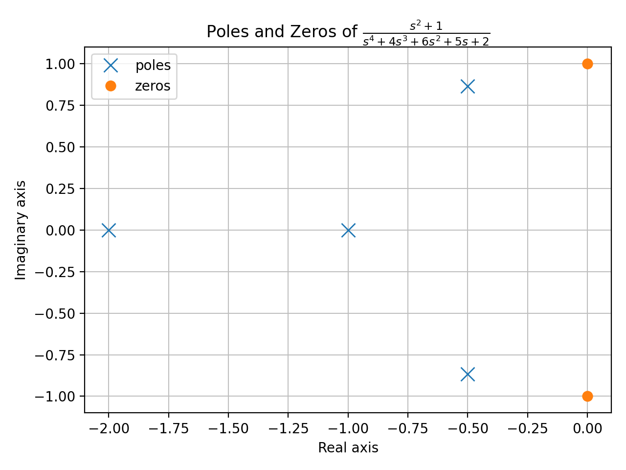
Returns the Pole-Zero plot (also known as PZ Plot or PZ Map) of a system.
A Pole-Zero plot is a graphical representation of a system’s poles and zeros. It is plotted on a complex plane, with circular markers representing the system’s zeros and ‘x’ shaped markers representing the system’s poles.
- Parameters:
- systemSISOLinearTimeInvariant type systems
The system for which the pole-zero plot is to be computed. It can be:
a single LTI SISO system.
a sequence of LTI SISO systems.
a sequence of 2-tuples
(LTI SISO system, label).a dict mapping LTI SISO systems to labels.
- pole_colorstr, tuple, optional
The color of the pole points on the plot.
- pole_markersizeNumber, optional
The size of the markers used to mark the poles in the plot. Default pole markersize is 10.
- zero_colorstr, tuple, optional
The color of the zero points on the plot.
- zero_markersizeNumber, optional
The size of the markers used to mark the zeros in the plot. Default zero markersize is 7.
- show_axesboolean, optional
If
True, the coordinate axes will be shown. Defaults to False.- z_rendering_kwdict
A dictionary of keyword arguments to further customize the appearance of zeros.
- p_rendering_kwdict
A dictionary of keyword arguments to further customize the appearance of poles.
- **kwargs
See
plotfor a list of keyword arguments to further customize the resulting figure.
References
Examples
>>> from sympy.abc import s
>>> from sympy.physics.control.lti import TransferFunction
>>> from spb import plot_pole_zero
>>> tf1 = TransferFunction(s**2 + 1, s**4 + 4*s**3 + 6*s**2 + 5*s + 2, s)
>>> plot_pole_zero(tf1)
Plot object containing:
[0]: 2D list plot
[1]: 2D list plot
(
Source code,png,hires.png,pdf)
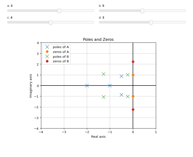
Interactive-widgets plot of multiple systems, one of which is parametric:
from sympy.abc import a, b, c, d, s
from sympy.physics.control.lti import TransferFunction
from spb import plot_pole_zero
tf1 = TransferFunction(s**2 + 1, s**4 + 4*s**3 + 6*s**2 + 5*s + 2, s)
tf2 = TransferFunction(s**2 + b, s**4 + a*s**3 + b*s**2 + c*s + d, s)
plot_pole_zero(
    (tf1, "A"), (tf2, "B"),
    params={
        a: (3, 0, 5),
        b: (5, 0, 10),
        c: (4, 0, 8),
        d: (3, 0, 5),
    },
    xlim=(-4, 1), ylim=(-4, 4),
    show_axes=True, use_latex=False)

- spb.control.plot_step_response(*systems, lower_limit=0, upper_limit=10, prec=8, show_axes=False, **kwargs)[source]
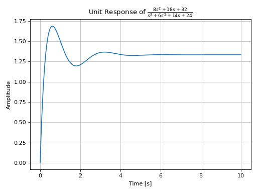
Returns the unit step response of a continuous-time system. It is the response of the system when the input signal is a step function.
- Parameters:
- systemSISOLinearTimeInvariant type
The LTI SISO system for which the Step Response is to be computed. It can be:
a single LTI SISO system.
a sequence of LTI SISO systems.
a sequence of 2-tuples
(LTI SISO system, label).a dict mapping LTI SISO systems to labels.
- lower_limitNumber, optional
The lower limit of the plot range. Defaults to 0.
- upper_limitNumber, optional
The upper limit of the plot range. Defaults to 10.
- precint, optional
The decimal point precision for the point coordinate values. Defaults to 8.
- show_axesboolean, optional
If
True, the coordinate axes will be shown. Defaults to False.- **kwargs
See
plotfor a list of keyword arguments to further customize the resulting figure.
See also
References
Examples
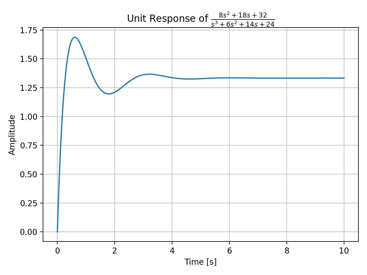
>>> from sympy.abc import s
>>> from sympy.physics.control.lti import TransferFunction
>>> from spb import plot_step_response
>>> tf1 = TransferFunction(8*s**2 + 18*s + 32, s**3 + 6*s**2 + 14*s + 24, s)
>>> plot_step_response(tf1)
(
Source code,png,hires.png,pdf)
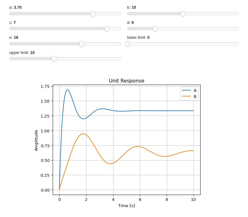
Interactive-widgets plot of multiple systems, one of which is parametric. Note the use of parametric
lower_limitandupper_limit.from sympy.abc import a, b, c, d, e, f, g, s from sympy.physics.control.lti import TransferFunction from spb import plot_step_response tf1 = TransferFunction(8*s**2 + 18*s + 32, s**3 + 6*s**2 + 14*s + 24, s) tf2 = TransferFunction(s**2 + a*s + b, s**3 + c*s**2 + d*s + e, s) plot_step_response( (tf1, "A"), (tf2, "B"), lower_limit=f, upper_limit=g, params={ a: (3.7, 0, 5), b: (10, 0, 20), c: (7, 0, 8), d: (6, 0, 25), e: (16, 0, 25), # NOTE: remove `None` if using ipywidgets f: (0, 0, 10, 50, None, "lower limit"), g: (10, 0, 25, 50, None, "upper limit"), }, use_latex=False)

- spb.control.plot_impulse_response(*systems, prec=8, lower_limit=0, upper_limit=10, show_axes=False, **kwargs)[source]
Returns the unit impulse response (Input is the Dirac-Delta Function) of a continuous-time system.
- Parameters:
- systemSISOLinearTimeInvariant type
The LTI SISO system for which the Impulse Response is to be computed. It can be:
a single LTI SISO system.
a sequence of LTI SISO systems.
a sequence of 2-tuples
(LTI SISO system, label).a dict mapping LTI SISO systems to labels.
- lower_limitNumber, optional
The lower limit of the plot range. Defaults to 0.
- upper_limitNumber, optional
The upper limit of the plot range. Defaults to 10.
- precint, optional
The decimal point precision for the point coordinate values. Defaults to 8.
- show_axesboolean, optional
If
True, the coordinate axes will be shown. Defaults to False.- **kwargs
See
plotfor a list of keyword arguments to further customize the resulting figure.
See also
References
Examples
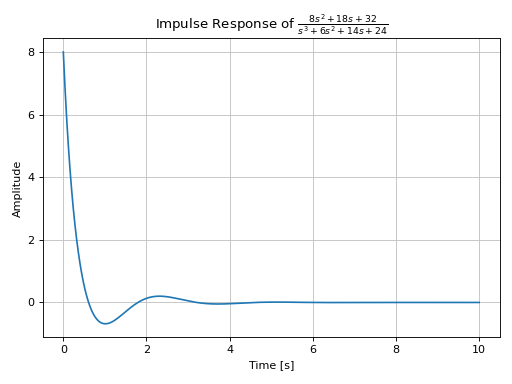
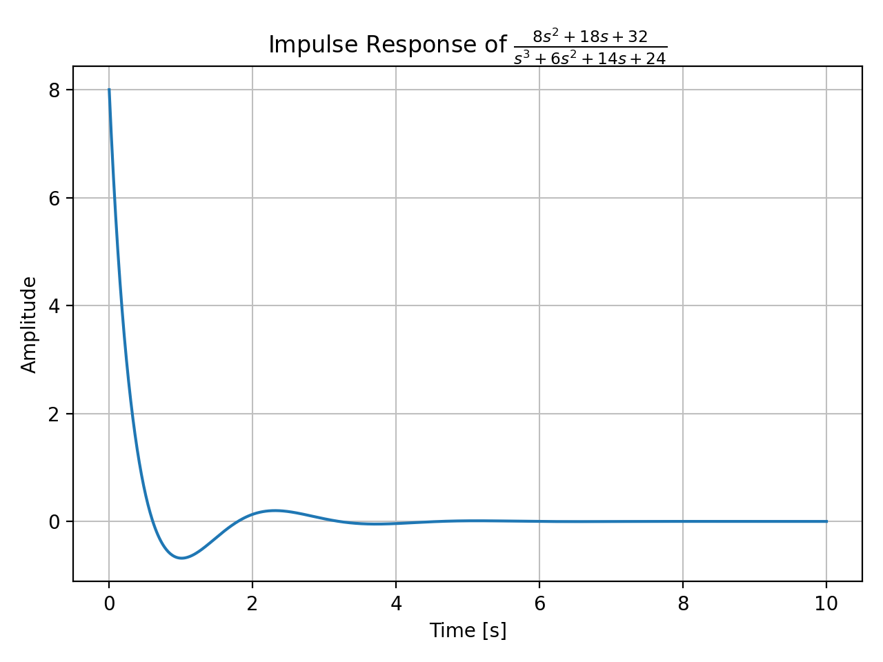
>>> from sympy.abc import s
>>> from sympy.physics.control.lti import TransferFunction
>>> from spb import plot_impulse_response
>>> tf1 = TransferFunction(8*s**2 + 18*s + 32, s**3 + 6*s**2 + 14*s + 24, s)
>>> plot_impulse_response(tf1)
(
Source code,png,hires.png,pdf)
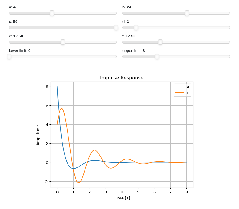
Interactive-widgets plot of multiple systems, one of which is parametric. Note the use of parametric
lower_limitandupper_limit.from sympy.abc import a, b, c, d, e, f, g, h, s from sympy.physics.control.lti import TransferFunction from spb import plot_impulse_response tf1 = TransferFunction(8*s**2 + 18*s + 32, s**3 + 6*s**2 + 14*s + 24, s) tf2 = TransferFunction(a*s**2 + b*s + c, s**3 + d*s**2 + e*s + f, s) plot_impulse_response( (tf1, "A"), (tf2, "B"), lower_limit=g, upper_limit=h, params={ a: (4, 0, 10), b: (24, 0, 40), c: (50, 0, 50), d: (3, 0, 25), e: (12.5, 0, 25), f: (17.5, 0, 50), # NOTE: remove `None` if using ipywidgets g: (0, 0, 10, 50, None, "lower limit"), h: (8, 0, 25, 50, None, "upper limit"), }, use_latex=False)

- spb.control.plot_ramp_response(*systems, slope=1, prec=8, lower_limit=0, upper_limit=10, show_axes=False, **kwargs)[source]
Returns the ramp response of a continuous-time system.
Ramp function is defined as the straight line passing through origin (\(f(x) = mx\)). The slope of the ramp function can be varied by the user and the default value is 1.
- Parameters:
- systemSISOLinearTimeInvariant type
The LTI SISO system for which the Ramp Response is to be computed. It can be:
a single LTI SISO system.
a sequence of LTI SISO systems.
a sequence of 2-tuples
(LTI SISO system, label).a dict mapping LTI SISO systems to labels.
- slopeNumber, optional
The slope of the input ramp function. Defaults to 1.
- lower_limitNumber, optional
The lower limit of the plot range. Defaults to 0.
- upper_limitNumber, optional
The upper limit of the plot range. Defaults to 10.
- precint, optional
The decimal point precision for the point coordinate values. Defaults to 8.
- show_axesboolean, optional
If
True, the coordinate axes will be shown. Defaults to False.- **kwargs
See
plotfor a list of keyword arguments to further customize the resulting figure.
See also
References
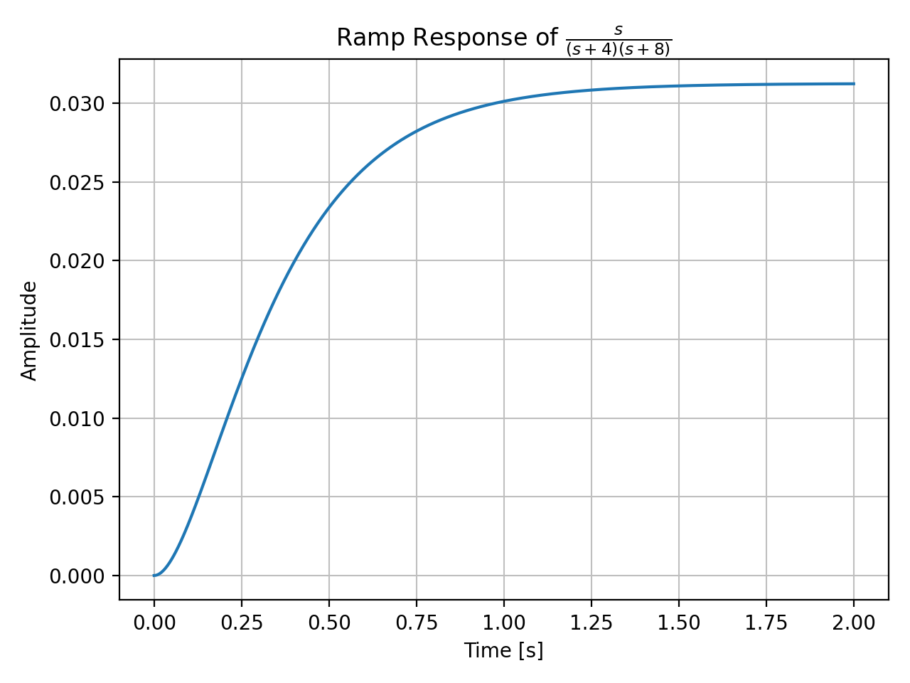
Examples
>>> from sympy.abc import s
>>> from sympy.physics.control.lti import TransferFunction
>>> from spb import plot_ramp_response
>>> tf1 = TransferFunction(s, (s+4)*(s+8), s)
>>> plot_ramp_response(tf1, upper_limit=2)
(
Source code,png,hires.png,pdf)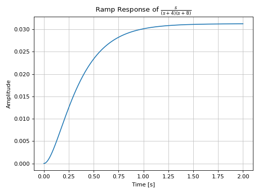
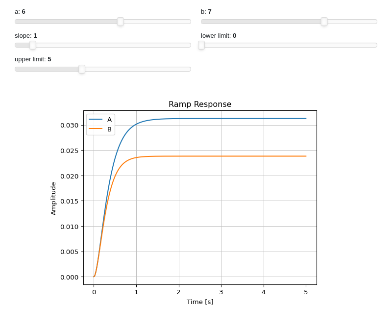
Interactive-widgets plot of multiple systems, one of which is parametric. Note the use of parametric
lower_limit,upper_limitandslope.from sympy.abc import a, b, c, d, e, s from sympy.physics.control.lti import TransferFunction from spb import plot_ramp_response tf1 = TransferFunction(s, (s+4)*(s+8), s) tf2 = TransferFunction(s, (s+a)*(s+b), s) plot_ramp_response( (tf1, "A"), (tf2, "B"), slope=c, lower_limit=d, upper_limit=e, params={ a: (6, 0, 10), b: (7, 0, 10), # NOTE: remove `None` if using ipywidgets c: (1, 0, 10, 50, None, "slope"), d: (0, 0, 5, 50, None, "lower limit"), e: (5, 2, 10, 50, None, "upper limit"), }, use_latex=False)
- spb.control.plot_bode_magnitude(*systems, initial_exp=-5, final_exp=5, freq_unit='rad/sec', show_axes=False, **kwargs)[source]
Returns the Bode magnitude plot of a continuous-time system.
See
plot_bodefor all the parameters.
- spb.control.plot_bode_phase(*systems, initial_exp=-5, final_exp=5, freq_unit='rad/sec', phase_unit='rad', show_axes=False, **kwargs)[source]
Returns the Bode phase plot of a continuous-time system.
See
plot_bodefor all the parameters.
- spb.control.plot_bode(*systems, initial_exp=-5, final_exp=5, freq_unit='rad/sec', phase_unit='rad', show_axes=False, **kwargs)[source]
Returns the Bode phase and magnitude plots of a continuous-time system.
- Parameters:
- systemSISOLinearTimeInvariant type
The LTI SISO system for which the Bode Plot is to be computed. It can be:
a single LTI SISO system.
a sequence of LTI SISO systems.
a sequence of 2-tuples
(LTI SISO system, label).a dict mapping LTI SISO systems to labels.
- initial_expNumber, optional
The initial exponent of 10 of the semilog plot. Defaults to -5.
- final_expNumber, optional
The final exponent of 10 of the semilog plot. Defaults to 5.
- precint, optional
The decimal point precision for the point coordinate values. Defaults to 8.
- show_axesboolean, optional
If
True, the coordinate axes will be shown. Defaults to False.- freq_unitstring, optional
User can choose between
'rad/sec'(radians/second) and'Hz'(Hertz) as frequency units.- phase_unitstring, optional
User can choose between
'rad'(radians) and'deg'(degree) as phase units.- unwrapbool, optional
Depending on the transfer function, there could be discontinuities in the phase plot. Set
unwrap=Trueto get a continuous phase. Default to False.- **kwargs
See
plotfor a list of keyword arguments to further customize the resulting figure.
See also
Examples
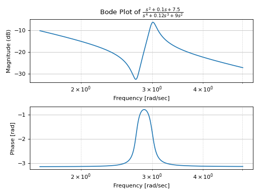
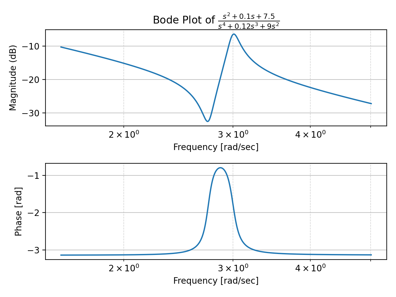
>>> from sympy.abc import s
>>> from sympy.physics.control.lti import TransferFunction
>>> from spb import plot_bode, plot_bode_phase, plotgrid
>>> tf1 = TransferFunction(1*s**2 + 0.1*s + 7.5, 1*s**4 + 0.12*s**3 + 9*s**2, s)
>>> plot_bode(tf1, initial_exp=0.2, final_exp=0.7)
(
Source code,png,hires.png,pdf)
In this example it is necessary to unwrap the phase:
>>> TransferFunction(1, s**3 + 2*s**2 + s, s)
>>> p1 = plot_bode_phase(tf, unwrap=False, show=False, title="unwrap=False")
>>> p2 = plot_bode_phase(tf, unwrap=True, show=False, title="unwrap=True")
>>> plotgrid(p1, p2)
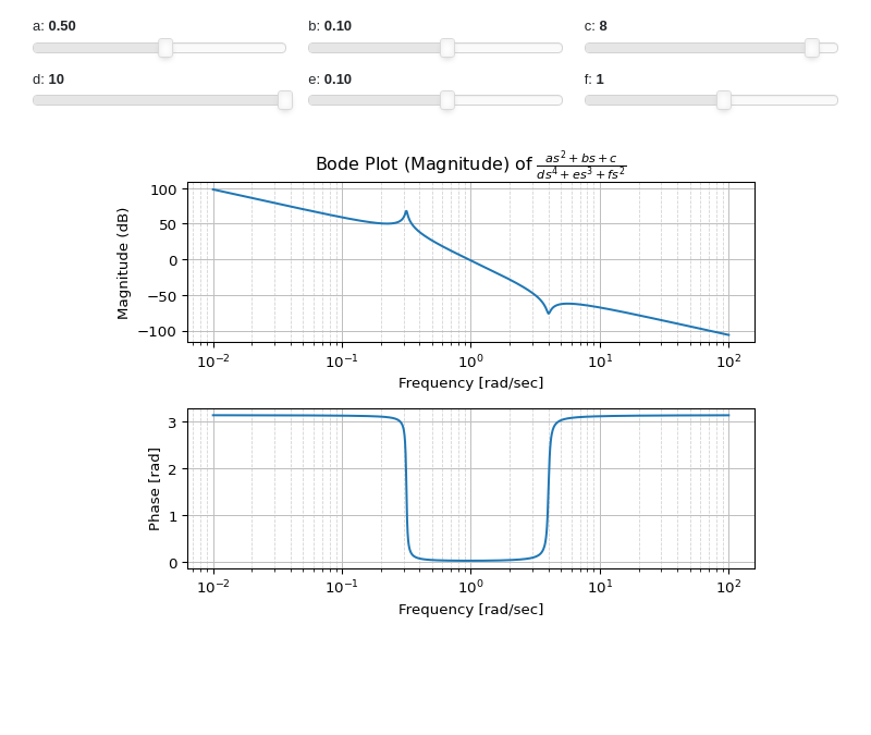
Interactive-widget plot:
from sympy.abc import a, b, c, d, e, f, s
from sympy.physics.control.lti import TransferFunction
from spb import *

tf1 = TransferFunction(a*s**2 + b*s + c, d*s**4 + e*s**3 + f*s**2, s)
plot_bode(
    tf1, initial_exp=-2, final_exp=2,
    params={
        a: (0.5, -10, 10),
        b: (0.1, -1, 1),
        c: (8, -10, 10),
        d: (10, -10, 10),
        e: (0.1, -1, 1),
        f: (1, -10, 10),
    },
    imodule="panel", ncols=3, use_latex=False
)

- spb.control.plot_nyquist(*systems, **kwargs)[source]
Nyquist plot for a system
Plots a Nyquist plot for the system over a (optional) frequency range. The curve is computed by evaluating the Nyqist segment along the positive imaginary axis, with a mirror image generated to reflect the negative imaginary axis. Poles on or near the imaginary axis are avoided using a small indentation. The portion of the Nyquist contour at infinity is not explicitly computed (since it maps to a constant value for any system with a proper transfer function).
- Parameters:
- systemSISOLinearTimeInvariant type
The LTI SISO system for which the Bode Plot is to be computed. It can be:
a single LTI SISO system.
a sequence of LTI SISO systems.
a sequence of 2-tuples
(LTI SISO system, label).a dict mapping LTI SISO systems to labels.
- arrowsint or 1D/2D array of floats, optional
Specify the number of arrows to plot on the Nyquist curve. If an integer is passed, that number of equally spaced arrows will be plotted on each of the primary segment and the mirror image. If a 1D array is passed, it should consist of a sorted list of floats between 0 and 1, indicating the location along the curve to plot an arrow.
- encirclement_thresholdfloat, optional
Define the threshold for generating a warning if the number of net encirclements is a non-integer value. Default value is 0.05.
- indent_directionstr, optional
For poles on the imaginary axis, set the direction of indentation to be ‘right’ (default), ‘left’, or ‘none’.
- indent_pointsint, optional
Number of points to insert in the Nyquist contour around poles that are at or near the imaginary axis.
- indent_radiusfloat, optional
Amount to indent the Nyquist contour around poles on or near the imaginary axis. Portions of the Nyquist plot corresponding to indented portions of the contour are plotted using a different line style.
- max_curve_magnitudefloat, optional
Restrict the maximum magnitude of the Nyquist plot to this value. Portions of the Nyquist plot whose magnitude is restricted are plotted using a different line style.
- max_curve_offsetfloat, optional
When plotting scaled portion of the Nyquist plot, increase/decrease the magnitude by this fraction of the max_curve_magnitude to allow any overlaps between the primary and mirror curves to be avoided.
- mirror_style[str, str] or [dict, dict] or dict or False, optional
Linestyles for mirror image of the Nyquist curve. If a list is given, the first element is used for unscaled portions of the Nyquist curve, the second element is used for portions that are scaled (using max_curve_magnitude). dict is a dictionary of keyword arguments to be passed to the plotting function, for example to plt.plot. If False then omit completely. Default linestyle is [’–’, ‘:’].
- m_circlesbool, optional
Turn on/off M-circles, which are circles of constant closed loop magnitude. Refer to [1] for more information.
- primary_style[str, str] or [dict, dict] or dict, optional
Linestyles for primary image of the Nyquist curve. If a list is given, the first element is used for unscaled portions of the Nyquist curve, the second element is used for portions that are scaled (using max_curve_magnitude). dict is a dictionary of keyword arguments to be passed to the plotting function, for example to Matplotlib’s plt.plot. Default linestyle is [‘-’, ‘-.’].
- omega_limitsarray_like of two values, optional
Limits to the range of frequencies.
- start_markerstr or dict, optional
Marker to use to mark the starting point of the Nyquist plot. If dict is provided, it must containts keyword arguments to be passed to the plot function, for example to Matplotlib’s plt.plot.
- warn_encirclementsbool, optional
If set to ‘False’, turn off warnings about number of encirclements not meeting the Nyquist criterion.
- **kwargs
See
plot_parametricfor a list of keyword arguments to further customize the resulting figure.
See also
Notes
If a continuous-time system contains poles on or near the imaginary axis, a small indentation will be used to avoid the pole. The radius of the indentation is given by indent_radius and it is taken to the right of stable poles and the left of unstable poles. If a pole is exactly on the imaginary axis, the indent_direction parameter can be used to set the direction of indentation. Setting indent_direction to none will turn off indentation. If return_contour is True, the exact contour used for evaluation is returned.
For those portions of the Nyquist plot in which the contour is indented to avoid poles, resuling in a scaling of the Nyquist plot, the line styles are according to the settings of the primary_style and mirror_style keywords. By default the scaled portions of the primary curve use a dotted line style and the scaled portion of the mirror image use a dashdot line style.
References
Examples
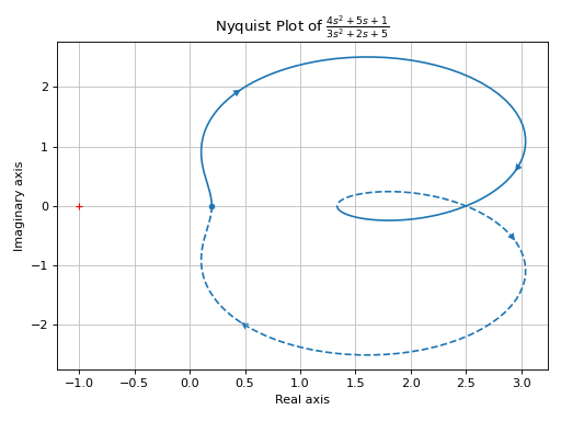
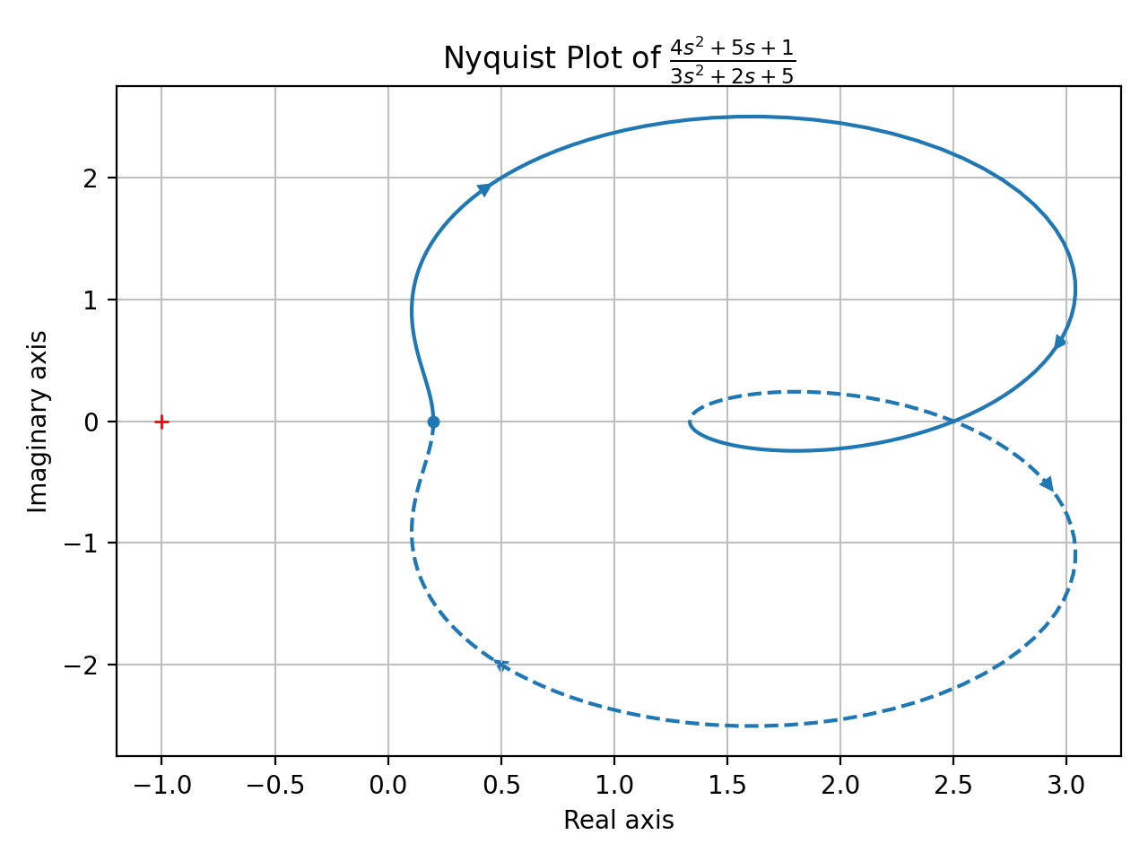
Plotting a single transfer function:
>>> from sympy import Rational
>>> from sympy.abc import s
>>> from sympy.physics.control.lti import TransferFunction
>>> from spb import plot_nyquist
>>> tf1 = TransferFunction(4 * s**2 + 5 * s + 1, 3 * s**2 + 2 * s + 5, s)
>>> plot_nyquist(tf1)
(
Source code,png,hires.png,pdf)
Visualizing M-circles:
>>> plot_nyquist(tf1, m_circles=True)
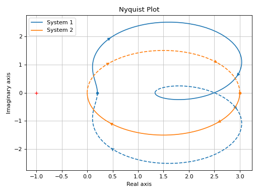
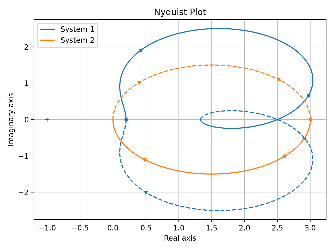
Plotting multiple transfer functions:
>>> tf2 = TransferFunction(1, s + Rational(1, 3), s)
>>> plot_nyquist(tf1, tf2)
(
Source code,png,hires.png,pdf)
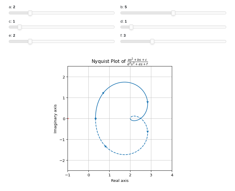
Interactive-widgets plot of a systems:
from sympy.abc import a, b, c, d, e, f, s
from sympy.physics.control.lti import TransferFunction
from spb import plot_nyquist
tf = TransferFunction(a * s**2 + b * s + c, d**2 * s**2 + e * s + f, s)
plot_nyquist(
    tf,
    params={
        a: (2, 0, 10),
        b: (5, 0, 10),
        c: (1, 0, 10),
        d: (1, 0, 10),
        e: (2, 0, 10),
        f: (3, 0, 10),
    },
    m_circles=False, use_latex=False,
    xlim=(-1, 4), ylim=(-2.5, 2.5), aspect="equal"
)
- spb.control.plot_nichols(*systems, **kwargs)[source]
Nichols plot for a system over a (optional) frequency range.
- Parameters:
- systemSISOLinearTimeInvariant type
The LTI SISO system for which the Bode Plot is to be computed. It can be:
a single LTI SISO system.
a sequence of LTI SISO systems.
a sequence of 2-tuples
(LTI SISO system, label).a dict mapping LTI SISO systems to labels.
- ngridbool, optional
Turn on/off the Nichols grid lines. Refer to [2] for more information.
- omega_limitsarray_like of two values, optional
Limits to the range of frequencies.
- **kwargs
See
plot_parametricfor a list of keyword arguments to further customize the resulting figure.
See also
References
Examples
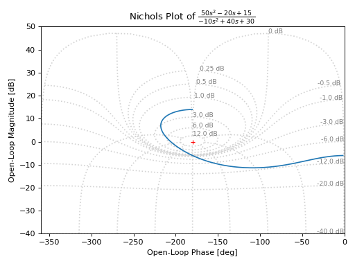
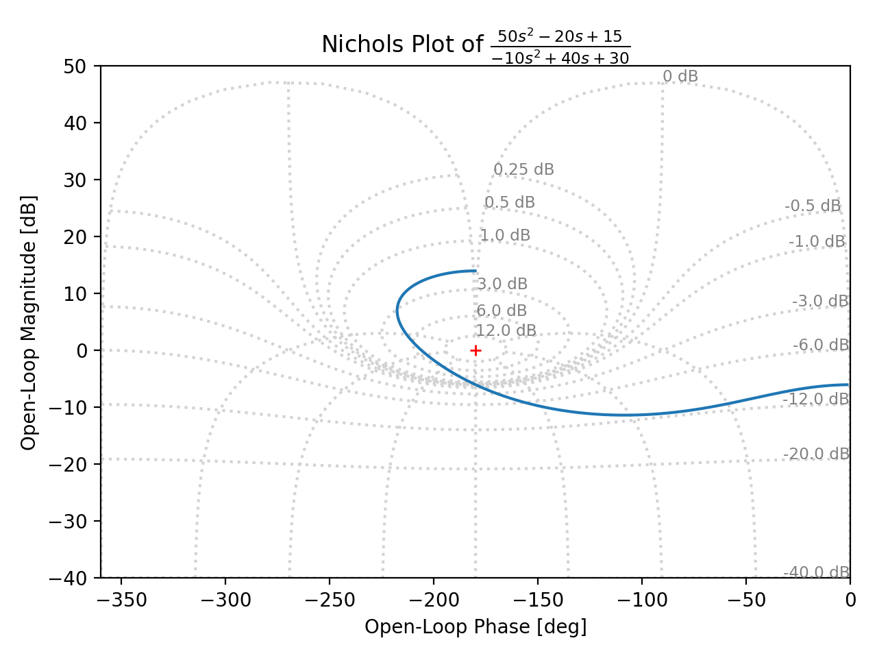
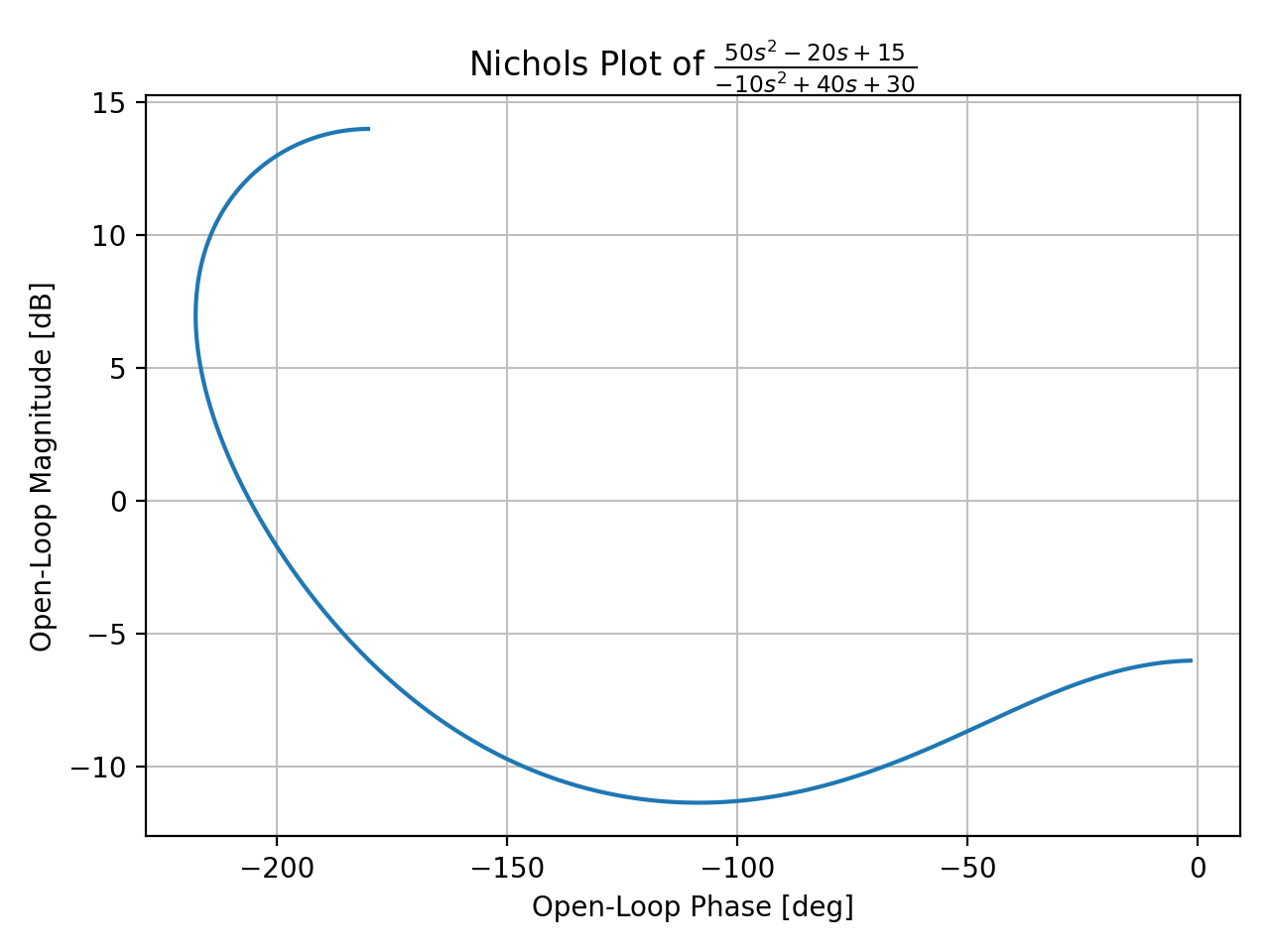
Plotting a single transfer function:
>>> from sympy.abc import s
>>> from sympy.physics.control.lti import TransferFunction
>>> from spb import plot_nichols
>>> tf = TransferFunction(50*s**2 - 20*s + 15, -10*s**2 + 40*s + 30, s)
>>> plot_nichols(tf)
(
Source code,png,hires.png,pdf)
Turning off the Nichols grid lines:
>>> plot_nichols(tf, ngrid=False)
(
Source code,png,hires.png,pdf)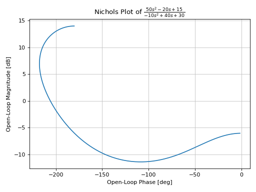
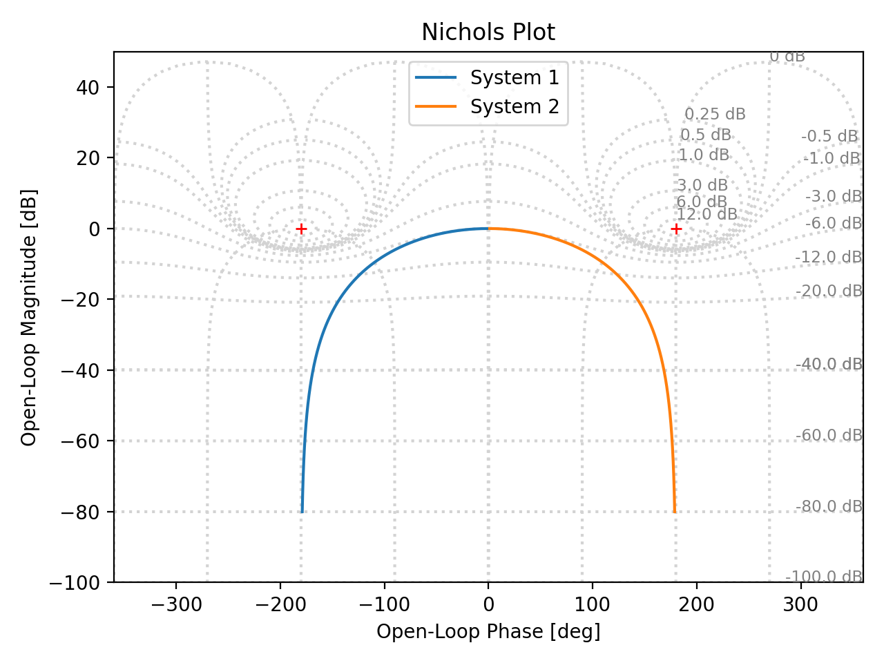
Plotting multiple transfer functions:
>>> tf1 = TransferFunction(1, s**2 + 2*s + 1, s)
>>> tf2 = TransferFunction(1, s**2 - 2*s + 1, s)
>>> plot_nichols(tf1, tf2, xlim=(-360, 360))
(
Source code,png,hires.png,pdf)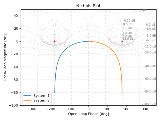
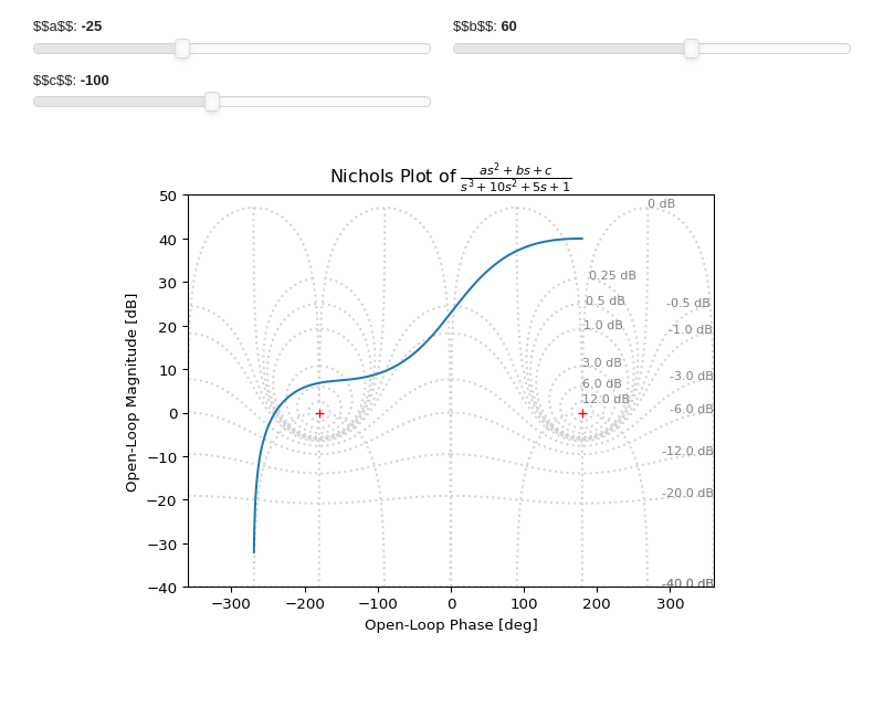
Interactive-widgets plot of a systems. For these kind of plots, it is recommended to set both
omega_limitsandxlim:from sympy.abc import a, b, c, s from spb import plot_nichols from sympy.physics.control.lti import TransferFunction tf = TransferFunction(a*s**2 + b*s + c, s**3 + 10*s**2 + 5 * s + 1, s) plot_nichols( tf, omega_limits=[1e-03, 1e03], n=1e04, params={ a: (-25, -100, 100), b: (60, -300, 300), c: (-100, -1000, 1000), }, xlim=(-360, 360) )
