plotgrid
- spb.plotgrid.plotgrid(*args, **kwargs)[source]
Combine multiple plots into a grid-like layout. This function has two modes of operation, depending on the input arguments. Make sure to read the examples to fully understand them.
- Parameters:
- argssequence
A sequence of aldready created plots. This, in combination with
nrandncrepresents the first mode of operation, where a basic grid with (nc * nr) subplots will be created.- nr, ncint, optional
Number of rows and columns. By default,
nc = 1andnr = -1: this will create as many rows as necessary, and a single column. By settingnr = 1a grid with a single row and as many columns as necessary will be created.- gsdict, optional
A dictionary mapping Matplotlib’s
GridSpecobjects to the plots. The keys represent the cells of the layout. Each cell will host the associated plot. This represents the second mode of operation, as it allows to create more complicated layouts.- imagegridboolean, optional
Requests Matplotlib’s
ImageGridaxes [2] to be used. This is best suited for plots with equal aspect ratio sharing a common colorbar. Default to False.- panel_kwdict, optional
A dictionary of keyword arguments to be passed to panel’s
GridSpecfor further customization. Default todict(sizing_mode="stretch_width"). Refer to [1] for more information.- showboolean, optional
It applies only to Matplotlib figures. Default to True.
- Returns:
- fig
plt.Figureorpn.GridSpec If all input plots are instances of
MatplotlibBackend, than a MatplotlibFigurewill be returned. Otherwise an instance of Holoviz Panel’sGridSpecwill be returned.
- fig
References
Examples
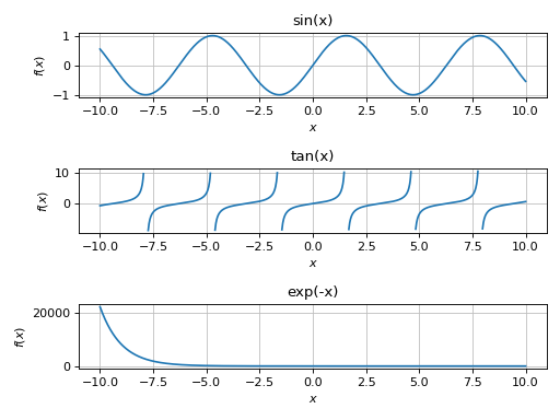
First mode of operation with instances of
MatplotlibBackend:from sympy import symbols, sin, cos, tan, exp, sqrt, Matrix, gamma, I from spb import * x, y, z = symbols("x, y, z") p1 = plot(sin(x), backend=MB, title="sin(x)", show=False) p2 = plot(tan(x), backend=MB, adaptive=False, detect_poles=True, title="tan(x)", show=False) p3 = plot(exp(-x), backend=MB, title="exp(-x)", show=False) plotgrid(p1, p2, p3)
(
Source code,png)
When plots represents images with equal aspect ratio and common colorbar, set
imagegrid=True:from sympy import symbols, sin, cos, pi, I from spb import * z = symbols("z") options = dict(coloring="b", show=False, grid=False) p1 = plot_complex(sin(z), (z, -pi-pi*I, pi+pi*I), **options) p2 = plot_complex(cos(z), (z, -pi-pi*I, pi+pi*I), **options) plotgrid(p1, p2, nr=1, imagegrid=True)
(
Source code,png)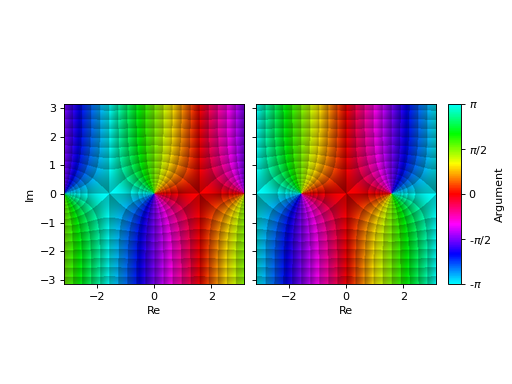
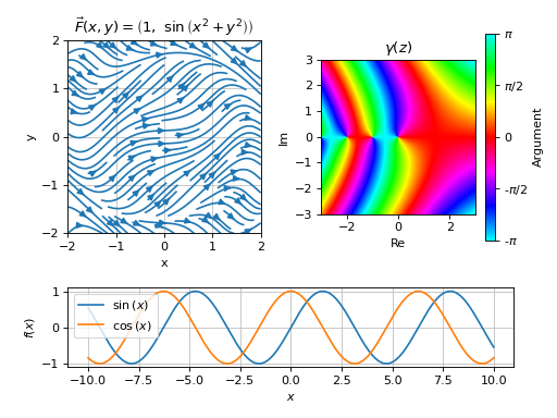
Second mode of operation, using Matplotlib
GridSpec:from sympy import * from spb import * from matplotlib.gridspec import GridSpec x, y, z = symbols("x, y, z") p1 = plot(sin(x), cos(x), adaptive=False, show=False) expr = Tuple(1, sin(x**2 + y**2)) p2 = plot_vector(expr, (x, -2, 2), (y, -2, 2), streamlines=True, scalar=False, use_cm=False, title=r"$\vec{F}(x, y) = %s$" % latex(expr), xlabel="x", ylabel="y", show=False) p3 = plot_complex(gamma(z), (z, -3-3*I, 3+3*I), title=r"$\gamma(z)$", grid=False, show=False) gs = GridSpec(3, 4) mapping = { gs[2, :]: p1, gs[0:2, 0:2]: p2, gs[0:2, 2:]: p3, } plotgrid(gs=mapping)
(
Source code,png)
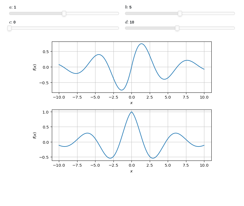
Interactive-widget plotgrid with first mode of operation, illustrating:
plotgridaccepts interactive plots.the use of the
prangeclass (parametric range).the same interactive module,
imodule, must be used on the plots as well as on the plotgrid. Here,imodule="panel"has been used, but users can change it toimodule="ipywidgets", provided that%matplotlib widgetis executed first.
from sympy import *
from spb import *
from sympy.abc import a, b, c, d, x
imodule = "panel"
options = dict(
    imodule=imodule, show=False, params={
        a: (1, 0, 2),
        b: (5, 0, 10),
        c: (0, 0, 2*pi),
        d: (10, 1, 20)
    })

p1 = plot(sin(x*a + c) * exp(-abs(x) / b), prange(x, -d, d), **options)
p2 = plot(cos(x*a + c) * exp(-abs(x) / b), (x, -10, 10), **options)
plotgrid(p1, p2, imodule=imodule)
