Interactive

The aim of this module is to quickly and easily create interactive widgets plots using either one of the following modules:

ipywidgets and ipympl: it probably has less dependencies to install and it might be a little bit faster at updating the visualization. However, it only works inside Jupyter Notebook.
Holoviz’s panel: works on any Python interpreter, as long as a browser is installed on the system. The interactive plot can be visualized directly in Jupyter Notebook, or in a new browser window where the plot can use the entire screen space. This might be useful to visualize plots with many parameters, or to focus the attention only on the plot rather than the code.

If only a minimal installation of this plotting module has been performed, then users have to manually install the chosen interactive modules.

By default, this plotting module will attempt to create interactive widgets with ipywidgets. To change interactive module, users can either:

specify the following keyword argument to use Holoviz’s Panel: imodule="panel". By default, the modules uses imodule="ipywidgets".
Modify the configuration file to permanently change the interactive module. More information are provided in 4 - Customizing the module.

To create an interactive widget plot, users have to provide the params= keyword argument to a plotting function, which must be a dictionary mapping parameters (SymPy’s symbols) to widgets. Let a, b, c, d be parameters. When imodule="panel", an example of params-dictionary is:

import panel as pn
params = {
    a: (1, 0, 5), # slider from 0 to 5, with default value of 1
    b: pn.widgets.FloatSlider(value=1, start=0, end=5), # same slider as above
    (c, d): pn.widgets.RangeSlider(value=(-1, 1), start=-3, end=3, step=0.1)
}

Or with imodule="ipywidgets":

import ipywidgets as w
params = {
    a: (1, 0, 5), # slider from 0 to 5, with default value of 1
    b: w.FloatSlider(value=1, min=0, max=5), # same slider as above
    (c, d): w.FloatRangeSlider(value=(-1, 1), min=-3, max=3, step=0.1)
}

From the above examples, it can be seen that the module requires widgets that returns numerical values. The code a: (1, 0, 5) is a shortcut to create a slider (more information down below). If a widget returns multiple numerical values (like panel.widgets.slider.RangeSlider or ipywidgets.widgets.widget_float.FloatRangeSlider), then a corresponding number of symbols must be provided.

Note that:

Interactive capabilities are already integrated with many plotting functions. The purpose of the following documentation is to show a few more examples for each interactive module.
It is not possible to mix ipywidgets and panel.
If the user is attempting to execute an interactive widget plot and gets an error similar to the following: TraitError: The ‘children’ trait of a Box instance contains an Instance of a TypedTuple which expected a Widget, not the FigureCanvasAgg at ‘0x…’. It means that the ipywidget module is being used with Matplotlib, but the interactive Matplotlib backend has not been loaded. First, execute the magic command %matplotlib widget, then execute the plot command.
For technical reasons, all interactive-widgets plots in this documentation are created using Holoviz’s Panel. Often, they will ran just fine with ipywidgets too. However, if a specific example uses the param library, or widgets from the panel module, then users will have to modify the params dictionary in order to make it work with ipywidgets. A couple of examples are provided below.

The prange class

class spb.utils.prange(*args)[source]

Represents a plot range, an entity describing what interval a particular variable is allowed to vary. It is a 3-elements tuple: (symbol, minimum, maximum).

Notes

Why does the plotting module needs this class instead of providing a plotting range with ordinary tuple/list? After all, ordinary plots works just fine.

If a plotting range is provided with a 3-elements tuple/list, the internal algorithm looks at the tuple and tries to determine what it is. If minimum and maximum are numeric values, than it is a plotting range.

Hovewer, there are some plotting functions in which the expression consists of 3-elements tuple/list. The plotting module is also interactive, meaning that minimum and maximum can also be expressions containing parameters. In these cases, the plotting range is indistinguishable from a 3-elements tuple describing an expression.

This class is meant to solve that ambiguity: it only represents a plotting range.

Examples

Let x be a symbol and u, v, t be parameters. An example plotting range is:

>>> from sympy import symbols
>>> from spb import prange
>>> x, u, v, t = symbols("x, u, v, t")
>>> prange(x, u * v, v**2 + t)
(x, u*v, t + v**2)

Holoviz’s panel

spb.interactive.panel.iplot(*series, show=True, **kwargs)[source]

Create an interactive application containing widgets and charts in order to study symbolic expressions, using Holoviz’s Panel for the user interace.

This function is already integrated with many of the usual plotting functions: since their documentation is more specific, it is highly recommended to use those instead.

However, the following documentation explains in details the main features exposed by the interactive module, which might not be included on the documentation of those other functions.

Parameters:

seriesBaseSeries

Instances of spb.series.BaseSeries, representing the symbolic expression to be plotted.

paramsdict

A dictionary mapping the symbols to a parameter. The parameter can be:

An instance of panel.widgets.base.Widget, something like panel.widgets.FloatSlider.
An instance of param.parameterized.Parameter.
A tuple with the form: (default, min, max, N, tick_format, label, spacing), which will instantiate a panel.widgets.FloatSlider or a panel.widgets.DiscreteSlider, depending on the spacing strategy. In particular:
- default, min, maxfloat
  Default value, minimum value and maximum value of the slider, respectively. Must be finite numbers. The order of these 3 numbers is not important: the module will figure it out which is what.
- Nint, optional
  Number of steps of the slider.
- tick_formatTickFormatter or None, optional
  Provide a formatter for the tick value of the slider. If None, panel will automatically apply a default formatter. Alternatively, an instance of bokeh.models.formatters.TickFormatter can be used. Default to None.
- label: str, optional
  Custom text associated to the slider.
- spacingstr, optional
  Specify the discretization spacing. Default to "linear", can be changed to "log".

Note that the parameters cannot be linked together (ie, one parameter cannot depend on another one).

layoutstr, optional

The layout for the controls/plot. Possible values:

'tb': controls in the top bar.
'bb': controls in the bottom bar.
'sbl': controls in the left side bar.
'sbr': controls in the right side bar.

If servable=False (plot shown inside Jupyter Notebook), then the default value is 'tb'. If servable=True (plot shown on a new browser window) then the default value is 'sbl'. Note that side bar layouts may not work well with some backends.

ncolsint, optional

Number of columns to lay out the widgets. Default to 2.

namestr, optional

The name to be shown on top of the interactive application, when served on a new browser window. Refer to servable to learn more. Default to an empty string.

pane_kwdict, optional

A dictionary of keyword/values which is passed to the pane containing the chart in order to further customize the output (read the Notes section to understand how the interactive plot is built). The following web pages shows the available options:

If Matplotlib is used, the figure is wrapped by panel.pane.plot.Matplotlib. Two interesting options are:
- interactive: wheter to activate the ipympl interactive backend.
- dpi: set the dots per inch of the output png. Default to 96.
If Plotly is used, the figure is wrapped by panel.pane.plotly.Plotly.
If Bokeh is used, the figure is wrapped by panel.pane.plot.Bokeh.

servablebool, optional

Default to False, which will show the interactive application on the output cell of a Jupyter Notebook. If True, the application will be served on a new browser window.

showbool, optional

Default to True. If True, it will return an object that will be rendered on the output cell of a Jupyter Notebook. If False, it returns an instance of InteractivePlot, which can later be be shown by calling the show() method.

templateoptional

Specify the template to be used to build the interactive application when servable=True. It can be one of the following options:

None: the default template will be used.
dictionary of keyword arguments to customize the default template. Among the options:
- full_width (boolean): use the full width of the browser page. Default to True.
- sidebar_width (str): CSS value of the width of the sidebar in pixel or %. Applicable only when layout='sbl' or layout='sbr'.
- show_header (boolean): wheter to show the header of the application. Default to True.
an instance of panel.template.base.BasicTemplate.
a subclass of panel.template.base.BasicTemplate.

titlestr or tuple

The title to be shown on top of the figure. To specify a parametric title, write a tuple of the form:(title_str, param_symbol1, ...), where:

title_str must be a formatted string, for example: "test = {:.2f}".
param_symbol1, ... must be a symbol or a symbolic expression whose free symbols are contained in the params dictionary.

throttledboolean, optional

Default to False. If True the recompute will be done at mouse-up event on sliders. If False, every slider tick will force a recompute.

use_latexbool, optional

Default to True. If True, the latex representation of the symbols will be used in the labels of the parameter-controls. If False, the string representation will be used instead.

See also

create_widgets

Notes

This function is specifically designed to work within Jupyter Notebook. It is also possible to use it from a regular Python console, by executing: iplot(..., servable=True), which will create a server process loading the interactive plot on the browser. However, spb.backends.k3d.K3DBackend is not supported in this mode of operation.
The interactive application consists of two main containers:
- a pane containing the widgets.
- a pane containing the chart, which can be further customize by setting the pane_kw dictionary. Please, read its documentation to understand the available options.
Some examples use an instance of bokeh.models.PrintfTickFormatter to format the value shown by a slider. This class is exposed by Bokeh, but can be used in interactive plots with any backend.
It has been observed that Dark Reader (or other night-mode-enabling browser extensions) might interfere with the correct behaviour of the output of interactive plots. Please, consider adding localhost to the exclusion list of such browser extensions.
spb.backends.matplotlib.MatplotlibBackend can be used, but the resulting figure is just a PNG image without any interactive frame. Thus, data exploration is not great. Therefore, the use of spb.backends.plotly.PlotlyBackend or spb.backends.bokeh.BokehBackend is encouraged.
When BokehBackend is used:
- rendering of gradient lines is slow.
- color bars might not update their ranges.

Examples

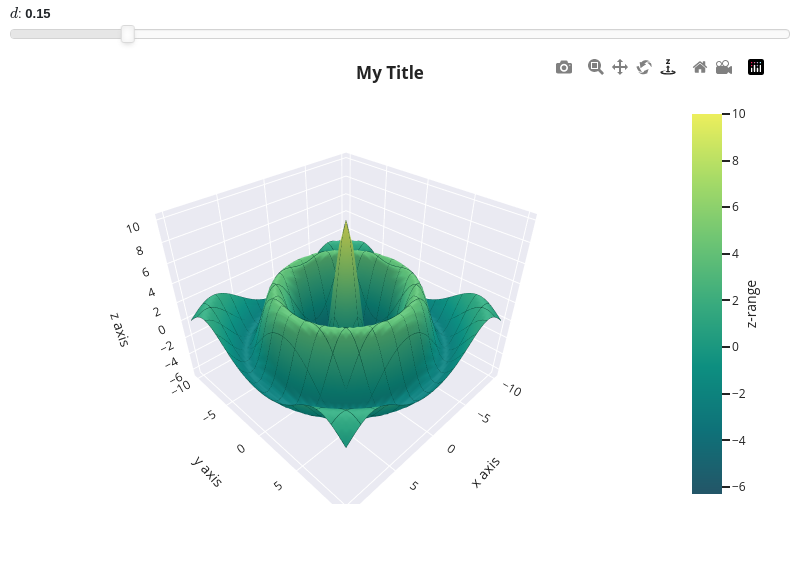
NOTE: the following examples use the ordinary plotting function because iplot is already integrated with them.

Surface plot between -10 <= x, y <= 10 discretized with 50 points on both directions, with a damping parameter varying from 0 to 1, and a default value of 0.15:

from sympy import *
from spb import *
x, y, z = symbols("x, y, z")
r = sqrt(x**2 + y**2)
d = symbols('d')
expr = 10 * cos(r) * exp(-r * d)
graphics(
    surface(
        expr, (x, -10, 10), (y, -10, 10), label="z-range",
        params={d: (0.15, 0, 1)}, n=51, use_cm=True,
        wireframe = True, wf_n1=15, wf_n2=15,
        wf_rendering_kw={"line_color": "#003428", "line_width": 0.75}
    ),
    title = "My Title",
    xlabel = "x axis",
    ylabel = "y axis",
    zlabel = "z axis",
    backend = PB
)

(Source code, small.png)

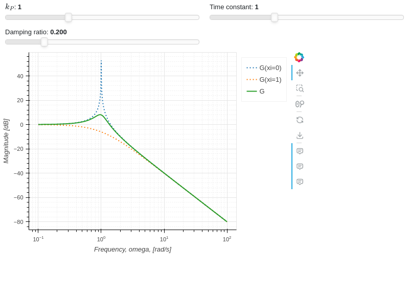
A line plot of the magnitude of a transfer function, illustrating the use of multiple expressions and:

some expression may not use all the parameters.
custom labeling of the expressions.
custom rendering of the expressions.
different ways to create sliders.
custom format of the value shown on the slider. This might be useful to correctly visualize very small or very big numbers.
custom labeling of the sliders.

from sympy import (symbols, sqrt, cos, exp, sin, pi, re, im,
    Matrix, Plane, Polygon, I, log)
from spb import *
from bokeh.models.formatters import PrintfTickFormatter
import panel as pn
import param
formatter = PrintfTickFormatter(format="%.3f")
kp, t, xi, o = symbols("k_P, tau, xi, omega")
G = kp / (I**2 * t**2 * o**2 + 2 * xi * t * o * I + 1)
mod = lambda x: 20 * log(sqrt(re(x)**2 + im(x)**2), 10)
plot(
    (mod(G.subs(xi, 0)), (o, 0.1, 100), "G(xi=0)", {"line_dash": "dotted"}),
    (mod(G.subs(xi, 1)), (o, 0.1, 100), "G(xi=1)", {"line_dash": "dotted"}),
    (mod(G), (o, 0.1, 100), "G"),
    params = {
        kp: (1, 0, 3),
        t: param.Number(default=1, bounds=(0, 3), label="Time constant"),
        xi: pn.widgets.FloatSlider(value=0.2, start=0, end=1,
            step=0.005, format=formatter, name="Damping ratio")
    },
    backend = BB,
    n = 2000,
    xscale = "log",
    xlabel = "Frequency, omega, [rad/s]",
    ylabel = "Magnitude [dB]",
)

(Source code, small.png)

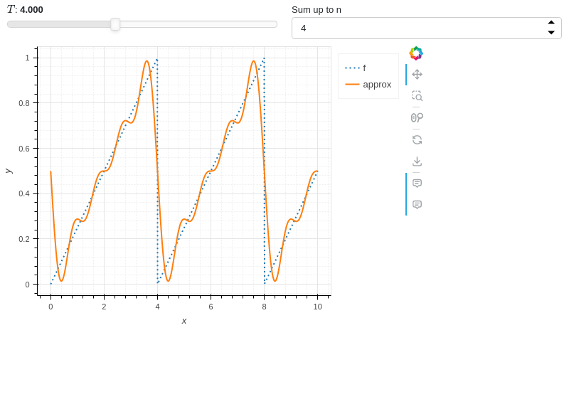
A line plot illustrating the Fouries series approximation of a saw tooth wave and:

custom format of the value shown on the slider.
creation of an integer spinner widget.

from sympy import *
from spb import *
import panel as pn
from bokeh.models.formatters import PrintfTickFormatter

x, T, n, m = symbols("x, T, n, m")
sawtooth = frac(x / T)
# Fourier Series of a sawtooth wave
fs = S(1) / 2 - (1 / pi) * Sum(sin(2 * n * pi * x / T) / n, (n, 1, m))

formatter = PrintfTickFormatter(format="%.3f")
plot(
    (sawtooth, (x, 0, 10), "f", {"line_dash": "dotted"}),
    (fs, (x, 0, 10), "approx"),
    params = {
        T: (4, 0, 10, 80, formatter),
        m: pn.widgets.IntInput(value=4, start=1, name="Sum up to n ")
    },
    xlabel = "x",
    ylabel = "y",
    backend = BB
)

(Source code, small.png)

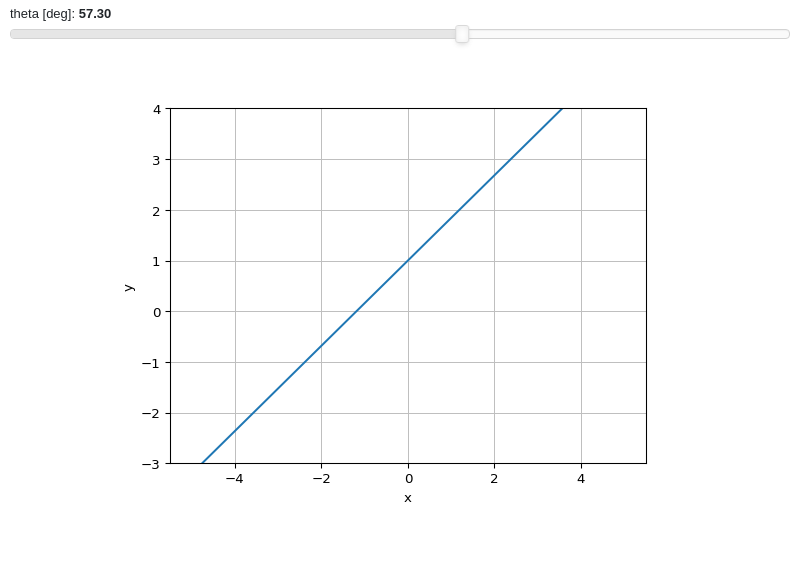
A line plot with a parameter representing an angle in radians, but showing the value in degrees on its label:

from sympy import sin, pi, symbols
from spb import *
from bokeh.models.formatters import CustomJSTickFormatter
# Javascript code is passed to `code=`
formatter = CustomJSTickFormatter(code="return (180./3.1415926 * tick).toFixed(2)")
x, t = symbols("x, t")

plot(
    (1 + x * sin(t), (x, -5, 5)),
    params = {
        t: (1, -2 * pi, 2 * pi, 100, formatter, "theta [deg]")
    },
    backend = MB,
    xlabel = "x", ylabel = "y",
    ylim = (-3, 4)
)

(Source code, small.png)

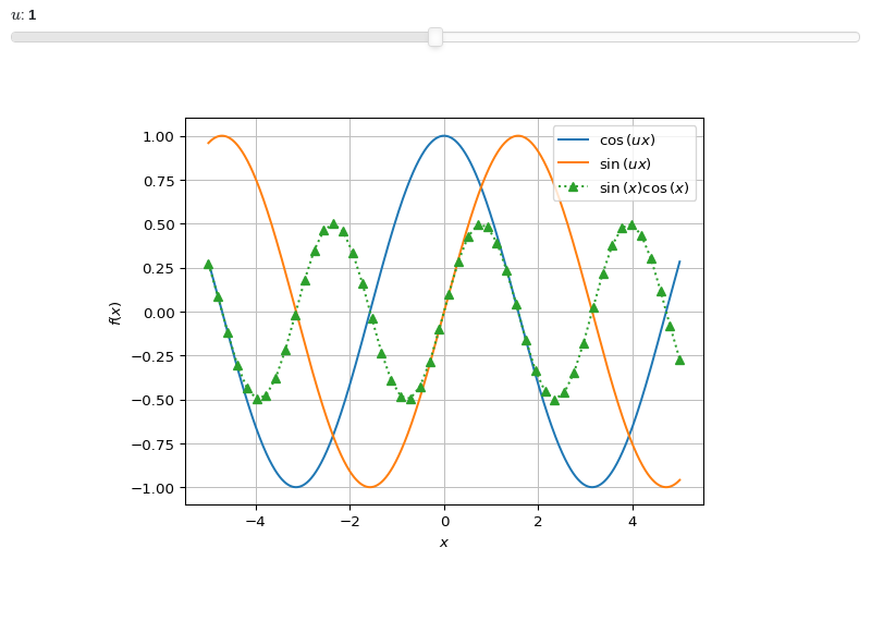
Combine together interactive and non interactive plots:

from sympy import sin, cos, symbols
from spb import *
x, u = symbols("x, u")
params = {
    u: (1, 0, 2)
}
graphics(
    line(cos(u * x), (x, -5, 5), params=params),
    line(sin(u * x), (x, -5, 5), params=params),
    line(
        sin(x)*cos(x), (x, -5, 5),
        rendering_kw={"marker": "^", "linestyle": ":"}, n=50),
)

(Source code, small.png)

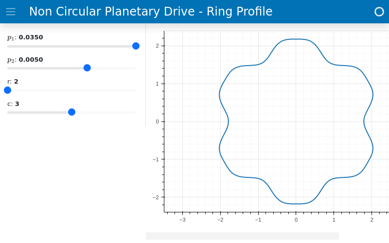
Serves the interactive plot to a separate browser window. Note that spb.backends.k3d.K3DBackend is not supported for this operation mode. Also note the two ways to create a integer sliders.

from sympy import *
from spb import *
import param
import panel as pn
from bokeh.models.formatters import PrintfTickFormatter
formatter = PrintfTickFormatter(format='%.4f')

p1, p2, t, r, c = symbols("p1, p2, t, r, c")
phi = - (r * t + p1 * sin(c * r * t) + p2 * sin(2 * c * r * t))
phip = phi.diff(t)
r1 = phip / (1 + phip)

plot_polar(
    (r1, (t, 0, 2*pi)),
    params = {
        p1: (0.035, -0.035, 0.035, 50, formatter),
        p2: (0.005, -0.02, 0.02, 50, formatter),
        # integer parameter created with param
        r: param.Integer(2, softbounds=(2, 5), label="r"),
        # integer parameter created with widgets
        c: pn.widgets.IntSlider(value=3, start=1, end=5, name="c")
    },
    backend = BB,
    aspect = "equal",
    n = 5000,
    layout = "sbl",
    ncols = 1,
    servable = True,
    name = "Non Circular Planetary Drive - Ring Profile"
)

(Source code, small.png)

ipywidgets

spb.interactive.ipywidgets.iplot(*series, show=True, **kwargs)[source]

Create an interactive application containing widgets and charts in order to study symbolic expressions, using ipywidgets.

This function is already integrated with many of the usual plotting functions: since their documentation is more specific, it is highly recommended to use those instead.

However, the following documentation explains in details the main features exposed by the interactive module, which might not be included on the documentation of those other functions.

Parameters:

seriesBaseSeries

Instances of spb.series.BaseSeries, representing the symbolic expression to be plotted.

paramsdict

A dictionary mapping the symbols to a parameter. The parameter can be:

a widget.
a tuple of the form: (default, min, max, N, tick_format, label, spacing), which will instantiate a ipywidgets.widgets.widget_float.FloatSlider or a ipywidgets.widgets.widget_float.FloatLogSlider, depending on the spacing strategy. In particular:
- default, min, maxfloat
  Default value, minimum value and maximum value of the slider, respectively. Must be finite numbers. The order of these 3 numbers is not important: the module will figure it out which is what.
- Nint, optional
  Number of steps of the slider.
- tick_formatstr or None, optional
  Provide a formatter for the tick value of the slider. Default to ".2f".
- label: str, optional
  Custom text associated to the slider.
- spacingstr, optional
  Specify the discretization spacing. Default to "linear", can be changed to "log".

Note that the parameters cannot be linked together (ie, one parameter cannot depend on another one).

layoutstr, optional

The layout for the controls/plot. Possible values:

'tb': controls in the top bar.
'bb': controls in the bottom bar.
'sbl': controls in the left side bar.
'sbr': controls in the right side bar.

The default value is 'tb'.

ncolsint, optional

Number of columns to lay out the widgets. Default to 2.

showbool, optional

Default to True. If True, it will return an object that will be rendered on the output cell of a Jupyter Notebook. If False, it returns an instance of InteractivePlot, which can later be shown by calling the show() method.

titlestr or tuple

The title to be shown on top of the figure. To specify a parametric title, write a tuple of the form:(title_str, param_symbol1, ...), where:

title_str must be a formatted string, for example: "test = {:.2f}".
param_symbol1, ... must be a symbol or a symbolic expression whose free symbols are contained in the params dictionary.

use_latexbool, optional

Default to True. If True, the latex representation of the symbols will be used in the labels of the parameter-controls. If False, the string representation will be used instead.

Notes

This function is specifically designed to work within Jupyter Notebook and requires the ipywidgets module .
To update Matplotlib plots, the %matplotlib widget command must be executed at the top of the Jupyter Notebook. It requires the installation of the ipympl module .

Examples

NOTE: the following examples use the ordinary plotting function because iplot is already integrated with them.

Surface plot between -10 <= x, y <= 10 discretized with 50 points on both directions, with a damping parameter varying from 0 to 1, and a default value of 0.15:

from sympy import *
from spb import *
x, y, z = symbols("x, y, z")
r = sqrt(x**2 + y**2)
d = symbols('d')
expr = 10 * cos(r) * exp(-r * d)
graphics(
    surface(
        expr, (x, -10, 10), (y, -10, 10), label="z-range",
        params={d: (0.15, 0, 1)}, n=51, use_cm=True,
        wireframe = True, wf_n1=15, wf_n2=15,
        wf_rendering_kw={"line_color": "#003428", "line_width": 0.75}
    ),
    title = "My Title",
    xlabel = "x axis",
    ylabel = "y axis",
    zlabel = "z axis",
    backend = PB,
    use_latex=False
)

A line plot illustrating how to specify widgets. In particular:

the parameter d will be rendered as a slider, with a custom formatter showing 3 decimal places.
the parameter n is a spinner.
the parameter phi will be rendered as a slider: note the custom number of steps and the custom label.
when using Matplotlib, the %matplotlib widget must be executed at the top of the notebook.

%matplotlib widget
from sympy import *
from spb import *
import ipywidgets

x, phi, n, d = symbols("x, phi, n, d")
plot(
    cos(x * n - phi) * exp(-abs(x) * d), (x, -5*pi, 5*pi),
    params={
        d: (0.1, 0, 1, ".3f"),
        n: ipywidgets.BoundedIntText(value=2, min=1, max=10,
            description="$n$"),
        phi: (0, 0, 2*pi, 50, r"$\phi$ [rad]")
    },
    ylim=(-1.25, 1.25))

A line plot illustrating the Fouries series approximation of a saw tooth wave and:

custom number of steps and label in the slider.
creation of an integer spinner widget.

from sympy import *
from spb import *
import ipywidgets

x, T, n, m = symbols("x, T, n, m")
sawtooth = frac(x / T)
# Fourier Series of a sawtooth wave
fs = S(1) / 2 - (1 / pi) * Sum(sin(2 * n * pi * x / T) / n, (n, 1, m))

plot(
    (sawtooth, (x, 0, 10), "f", {"line_dash": "dotted"}),
    (fs, (x, 0, 10), "approx"),
    params = {
        T: (4, 0, 10, 80, "Period, T"),
        m: ipywidgets.BoundedIntText(value=4, min=1, max=100,
            description="Sum up to n ")
    },
    xlabel = "x",
    ylabel = "y",
    backend = BB
)

A line plot of the magnitude of a transfer function, illustrating the use of multiple expressions and:

some expression may not use all the parameters.
custom labeling of the expressions.
custom rendering of the expressions.
custom number of steps in the slider.
custom labeling of the parameter-sliders.

from sympy import (symbols, sqrt, cos, exp, sin, pi, re, im,
    Matrix, Plane, Polygon, I, log)
from spb import *
kp, t, z, o = symbols("k_P, tau, zeta, omega")
G = kp / (I**2 * t**2 * o**2 + 2 * z * t * o * I + 1)
mod = lambda x: 20 * log(sqrt(re(x)**2 + im(x)**2), 10)
plot(
    (mod(G.subs(z, 0)), (o, 0.1, 100), "G(z=0)", {"line_dash": "dotted"}),
    (mod(G.subs(z, 1)), (o, 0.1, 100), "G(z=1)", {"line_dash": "dotted"}),
    (mod(G), (o, 0.1, 100), "G"),
    params = {
        kp: (1, 0, 3),
        t: (1, 0, 3),
        z: (0.2, 0, 1, 200, "z")
    },
    backend = BB,
    n = 2000,
    xscale = "log",
    xlabel = "Frequency, omega, [rad/s]",
    ylabel = "Magnitude [dB]",
)

A polar line plot. Note:

when using Matplotlib, the %matplotlib widget must be executed at the top of the notebook.
the two ways to create a integer sliders.

%matplotlib widget
from sympy import *
from spb import *
import ipywidgets

p1, p2, t, r, c = symbols("p1, p2, t, r, c")
phi = - (r * t + p1 * sin(c * r * t) + p2 * sin(2 * c * r * t))
phip = phi.diff(t)
r1 = phip / (1 + phip)

plot_polar(
    (r1, (t, 0, 2*pi)),
    params = {
        p1: (0.035, -0.035, 0.035, 50),
        p2: (0.005, -0.02, 0.02, 50),
        # integer parameter created with ipywidgets
        r: ipywidgets.BoundedIntText(value=2, min=2, max=5,
            description="r"),
        # integer parameter created with usual syntax
        c: (3, 1, 5, 4)
    },
    backend = MB,
    aspect = "equal",
    n = 5000,
    name = "Non Circular Planetary Drive - Ring Profile"
)

Combine together interactive and non interactive plots:

from sympy import sin, cos, symbols
from spb import *
x, u = symbols("x, u")
params = {
    u: (1, 0, 2)
}
graphics(
    line(cos(u * x), (x, -5, 5), params=params),
    line(sin(u * x), (x, -5, 5), params=params),
    line(
        sin(x)*cos(x), (x, -5, 5),
        rendering_kw={"marker": "^", "linestyle": ":"}, n=50),
)