3 - Differences between 3D backends
NOTE: there is an html link above some of the pictures in this page: click
it to load the html page containing the plot and interact with it.
In this tutorial we are going to compare the same plot produced with 3 different backends. In particular, we will focus on usability and interactivity.
First, let’s initialize the tutorial by running:
%matplotlib widget
from sympy import *
from spb import *
u, v = symbols("u, v")
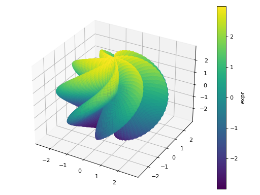
Now, let’s visualize a plot created with Matplotlib:
from sympy import *
from spb import *
u, v = symbols("u, v")
r = 2 + sin(7 * u + 5 * v)
expr = (
    r * cos(u) * sin(v),
    r * sin(u) * sin(v),
    r * cos(v)
)
plot3d_parametric_surface(*expr, (u, 0, 2 * pi), (v, 0, pi), "expr",
    backend=MB, use_cm=True)
(Source code, png)

Here, we can guess what the exact shape of the surface is going to be. We could increase the number of discretization points, in the u and v directions, but we are not going to do that with Matplotlib, as the rendering would become excessively slow. As always, we can use the toolbar buttons to zoom in and out. Now, try to click and drag the surface: there is a lot of lag. Matplotlib is not designed to be interactive.
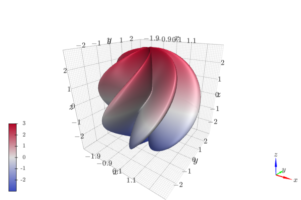
Let’s plot the same surface with K3D-Jupyter. Since we are at it, let’s
also bump up the number of discretization points to 250 on both parameters.
The resulting mesh will have 62500 points, therefore the computation
may take a few seconds (depending on our machine). Note one major difference
with SymPy’s plotting module: to specify the same numer of discretization points on both directions we can use the keyword argument n.
Alternatively, we could use n1 and n2 to specify different numbers
of discretization points.
from sympy import *
from spb import *
u, v = symbols("u, v")
n = 250
r = 2 + sin(7 * u + 5 * v)
expr = (
    r * cos(u) * sin(v),
    r * sin(u) * sin(v),
    r * cos(v)
)
plot3d_parametric_surface(*expr, (u, 0, 2 * pi), (v, 0, pi), "expr",
    n=n, backend=KB, use_cm=True)

To interact with the plot:
Left click and drag: rotate the plot.
Scroll with the mouse wheel: zoom in and out.
Right click and drag: pan.
Note how smooth the interaction is!!!
On the top right corner there is a menu with a few entries:
Controls: we can play with a few options, like hiding the grids, going full screen, …, add and remove clipping planes.
Objects: we can see the objects displayed on the plot. Let’s click the
Mesh #1entry: we can hide/show the object, its color legend, we can turn on wireframe view (don’t do it with such a high number of points, it will slows things down a lot!). Note that by default a color map is applied to the surface, hence we cannot change its color. To apply a solid color to the mesh, run again the previous command also providing theuse_cm=Falsekeyword argument.Info: useful information for debug purposes.
It is left to the Reader to play with the controls and learn what they do.
Note that the name of the surface displayed under Objects is Mesh #1.
If we plot multiple expressions, the names will be Mesh #1,
Mesh #2, … This is the default behaviour for K3DBackend.
We can also chose to display the string representation of the expression by
setting show_label=True, but it is safe to assume that the label won’t fit the small amount of width of the Controls user interface, therefore it makes sense to leave that option unset.
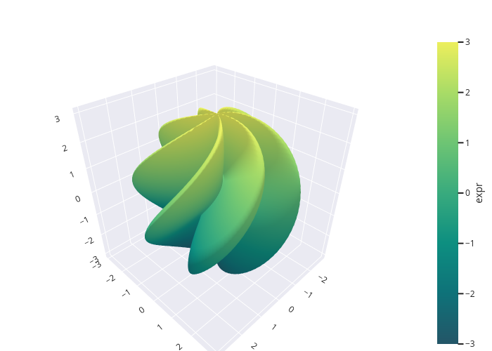
Finally, let’s look at the same plot with Plotly:
from sympy import *
from spb import *
u, v = symbols("u, v")
r = 2 + sin(7 * u + 5 * v)
expr = (
    r * cos(u) * sin(v),
    r * sin(u) * sin(v),
    r * cos(v)
)
n = 150
plot3d_parametric_surface(*expr, (u, 0, 2 * pi), (v, 0, pi), "expr",
    n=n, backend=PB, use_cm=True)
(Source code, png)
Plotly is also great with 3D plots. The main difference between Plotly and K3D-Jupyter are:
the former can stretch the axis, whereas the latter (being more engineering-oriented) uses a fixed aspect ratio representing reality. Type
help(PB)to understand how to control the aspect ratio of Plotly.Plotly is consistently slower at rendering 3D objects than K3D-Jupyter.
Plotly doesn’t natively support wireframe.
By moving the cursor over the surface, we can actually see the coordinates of the “selected” point. This is not currently possible with
K3DBackend.