3 - Customizing the module
Let’s suppose we have identified two backends that we like (one for 2D plots,
the other for 3D plots). Then, instead of providing the keyword
backend=SOMETHING each time we need to create a plot, we can customize the
module to make the plotting functions use our backends. Moreso, it is also
possible to customize the appearance of the backends.
Let’s import the necessary tools and visualize the current settings:
from spb.defaults import cfg, set_defaults
display(cfg)
Here, we can see the settings associated to the 4 backends: 'plotly',
'bokeh', 'matplotlib', 'k3d'. We will discuss each option later on.
Let’s learn how to use the set_defaults function:
help(set_defaults)
We need to change the values in the cfg dictionary and then use the
set_defaults function to apply the new configurations.
Let’s say we would like to:
use Plotly for 2D plots and Matplotlib for 3D plots;
use
"seaborn"theme in Plotly. We can use help(PB) (or any other backend) to read the documentation associated to each backend, in which we will find links towards the official documentation of the plotting library, where we will find the available themes.
Then:
# we write the name of the plotting library
# available options: bokeh, matplotlib, k3d, plotly
cfg["backend_2D"] = "plotly"
cfg["backend_3D"] = "matplotlib"
# the following depends on the plotting library
cfg["plotly"]["theme"] = "seaborn"
set_defaults(cfg)
Note that if we insert invalid options, the module will automatically reset to the default settings!
Now, let’s restart the kernel in order to make changes effective. Then, we can test test them right away.
from sympy import *
from spb import *
var("u, v, x, y")
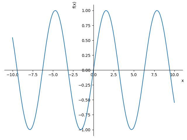
plot(sin(x), cos(x), log(x))
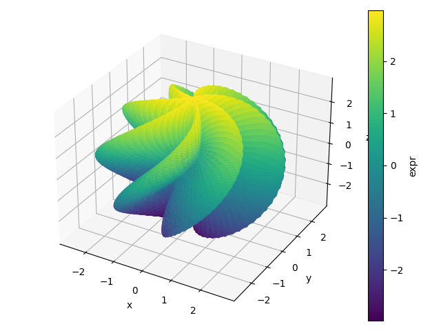
n = 125
r = 2 + sin(7 * u + 5 * v)
expr = (
    r * cos(u) * sin(v),
    r * sin(u) * sin(v),
    r * cos(v)
)
plot3d_parametric_surface(*expr, (u, 0, 2 * pi), (v, 0, pi), "expr", n=n)
Available Options
Let’s now discuss a few customization options:
# Set the location of the intersection between the horizontal and vertical
# axis of Matplotlib (only works for 2D plots). Possible values:
#       "center", "auto" or None
# If None, use a standard Matplotlib layout with vertical axis on the left,
# horizontal axis on the bottom.
cfg["matplotlib"]["axis_center"] = None
# Turn on the grid on Matplotlib figures
cfg["matplotlib"]["grid"] = True
# Show minor grids
cfg["matplotlib"]["show_minor_grid"] = True

# Find more Plotly themes at the following page:
# https://plotly.com/python/templates/
cfg["plotly"]["theme"] = "seaborn"
# Turn on the grid on Plotly figures
cfg["plotly"]["grid"] = True

# Find more Bokeh themes at the following page:
# https://docs.bokeh.org/en/latest/docs/reference/themes.html
cfg["bokeh"]["theme"] = "caliber"
# Activate automatic update event on panning
cfg["bokeh"]["update_event"] = True
# Turn on the grid on Bokeh figures
cfg["bokeh"]["grid"] = True
# Show minor grids
cfg["bokeh"]["show_minor_grid"] = True
# depending on the used Bokeh `themes`, we will need
# to adjust the opacity of the minor grid lines
cfg["bokeh"]["minor_grid_line_alpha"] = 0.6
# controls the spacing of the dashes in minor grid lines
cfg["bokeh"]["minor_grid_line_dash"] = [2, 2]

# Turn on the grid on K3D-Jupyter figures
cfg["k3d"]["grid"] = True
# K3D-Jupyter colors are represented by an integer number.
cfg["k3d"]["bg_color"] = 0xffffff
cfg["k3d"]["grid_color"] = 0xE6E6E6
cfg["k3d"]["label_color"] = 0x444444

# we can set the numerical evaluation library for complex plots.
# Available options: "mpmath" or None (the latter uses Numpy/Scipy)
cfg["complex"]["modules"] = None
# set a default (complex) domain coloring option.
cfg["complex"]["coloring"] = "b"

# Visualize Latex labels in the widgets of `iplot`
cfg["interactive"]["use_latex"] = True
# Controls wether sliders trigger the update of `iplot`at each
# tick (value False) or only when the mouse click is released
# (value True)
cfg["interactive"]["throttled"] = False

# Set the default evaluation algorithm for line plots:
# True: use adaptive algorithm
# False: use uniform mesh algorithm
cfg["adaptive"]["used_by_default"] = True
# Set the "smoothness" goal for the adaptive algorithm.
# Lower values create smoother lines, at the cost of
# performance.
cfg["adaptive"]["goal"] = 0.01

# Set the overall plot range to be used when the plotting
# variable is not specified.
cfg["plot_range"]["min"] = -10
cfg["plot_range"]["max"] = 10
Let’s consider MatplotlibBackend. Let’s suppose we would like to use
the old plotting module style:
plot(sin(x), backend=MB, axis_center="auto", grid=False)
Then, we can modify the cfg dictionary and execute the set_defaults
function, finally restarting the kernel to make the changes effective.
Resetting the configuration file
Suppose we would like to go back to the original default settings. Then:
from spb.defaults import reset
reset()
Now, we restart the kernel and the plotting module is back at its original state.