Complex
NOTE:
For technical reasons, all interactive-widgets plots in this documentation are
created using Holoviz’s Panel. Often, they will ran just fine with ipywidgets
too. However, if a specific example uses the param library, then users
will have to modify the params dictionary in order to make it work with
ipywidgets. Refer to Interactive module for more information.
- spb.ccomplex.complex.plot_complex(*args, **kwargs)[source]
Plot the absolute value of a complex function colored by its argument. By default, the aspect ratio of 2D plots is set to
aspect="equal".Depending on the provided range, this function will produce different types of plots:
Line plot over the reals.
Image plot over the complex plane if
threed=False. This is also known as Domain Coloring. Use thecoloringkeyword argument to select a different coloring strategy andcmapto set a custom color map (default to HSV).If
threed=True, plot a 3D surface of the absolute value over the complex plane, colored by its argument. Use thecoloringkeyword argument to select a different coloring strategy andcmapto set a custom color map (default to HSV).
Read the Notes section to learn more about colormaps.
Typical usage examples are in the followings:
- Plotting a single expression with a single range.
plot_complex(expr, range, **kwargs)
- Plotting a single expression with the default range (-10, 10).
plot_complex(expr, **kwargs)
- Plotting multiple expressions with a single range.
plot_complex(expr1, expr2, …, range, **kwargs)
- Plotting multiple expressions with multiple ranges.
plot_complex((expr1, range1), (expr2, range2), …, **kwargs)
- Plotting multiple expressions with custom labels and rendering options.
plot_complex((expr1, range1, label1, rendering_kw1), (expr2, range2, label2, rendering_kw2), …, **kwargs)
- Parameters:
- args
- exprExpr or callable
Represent the complex function to be plotted. It can be a:
Symbolic expression.
Numerical function of one variable, supporting vectorization. In this case the following keyword arguments are not supported:
params.
- range3-element tuple
Denotes the range of the variables. For example:
(z, -5, 5): plot a line over the reals from point -5 to 5(z, -5 + 2*I, 5 + 2*I): plot a line from complex point(-5 + 2*I)to(5 + 2 * I). Note the same imaginary part for the start/end point. Also note that we can specify the ranges by using standard Python complex numbers, for example(z, -5+2j, 5+2j).(z, -5 - 3*I, 5 + 3*I): surface or contour plot of the complex function over the specified domain.
- labelstr, optional
The name of the complex function to be eventually shown on the legend. If none is provided, the string representation of the function will be used.
- rendering_kwdict, optional
A dictionary of keywords/values which is passed to the backend’s function to customize the appearance of lines, surfaces or images. Refer to the plotting library (backend) manual for more informations.
- adaptivebool, optional
If
True, creates line plots by using an adaptive algorithm. Useadaptive_goalandloss_fnto further customize the output. Image and surface plots do not use an adaptive algorithm.Default to
False, which uses a uniform sampling strategy.- adaptive_goalcallable, int, float or None
Controls the “smoothness” of the evaluation. Possible values:
None(default): it will use the following goal:lambda l: l.loss() < 0.01number (int or float). The lower the number, the more evaluation points. This number will be used in the following goal:
lambda l: l.loss() < numbercallable: a function requiring one input element, the learner. It must return a float number. Refer to [2] for more information.
- aspect(float, float) or str, optional
Set the aspect ratio of the plot. The value depends on the backend being used. Read that backend’s documentation to find out the possible values.
- at_infinityboolean, optional
Apply the transformation \(z \rightarrow \frac{1}{z}\) in order to study the behaviour of the function around the point at infinity. It is recommended to also set
axis=Falsein order to avoid confusion.- backendPlot, optional
A subclass of
Plot, which will perform the rendering. Default toMatplotlibBackend.- blevelfloat, optional
Controls the black level of ehanced domain coloring plots. It must be 0 (black) <= blevel <= 1 (white). Default to 0.75.
- cmapstr, iterable, optional
Specify the colormap to be used on enhanced domain coloring plots (both images and 3d plots). Default to
"hsv". Can be any colormap from matplotlib or colorcet.- colorbarboolean, optional
Show/hide the colorbar. Default to True (colorbar is visible).
- coloringstr or callable, optional
Choose between different domain coloring options. Default to
"a". Refer to [1] for more information."a": standard domain coloring showing the argument of the complex function."b": enhanced domain coloring showing iso-modulus and iso-phase lines."c": enhanced domain coloring showing iso-modulus lines."d": enhanced domain coloring showing iso-phase lines."e": alternating black and white stripes corresponding to modulus."f": alternating black and white stripes corresponding to phase."g": alternating black and white stripes corresponding to real part."h": alternating black and white stripes corresponding to imaginary part."i": cartesian chessboard on the complex points space. The result will hide zeros."j": polar Chessboard on the complex points space. The result will show conformality."k": black and white magnitude of the complex function. Zeros are black, poles are white."l":enhanced domain coloring showing iso-modulus and iso-phase lines, blended with the magnitude: white regions indicates greater magnitudes. Can be used to distinguish poles from zeros."m": enhanced domain coloring showing iso-modulus lines, blended with the magnitude: white regions indicates greater magnitudes. Can be used to distinguish poles from zeros."n": enhanced domain coloring showing iso-phase lines, blended with the magnitude: white regions indicates greater magnitudes. Can be used to distinguish poles from zeros."o": enhanced domain coloring showing iso-phase lines, blended with the magnitude: white regions indicates greater magnitudes. Can be used to distinguish poles from zeros.
The user can also provide a callable,
f(w), wherewis an [n x m] Numpy array (provided by the plotting module) containing the results (complex numbers) of the evaluation of the complex function. The callable should return:- imgndarray [n x m x 3]
An array of RGB colors (0 <= R,G,B <= 255)
- colorscalendarray [N x 3] or None
An array with N RGB colors, (0 <= R,G,B <= 255). If
colorscale=None, no color bar will be shown on the plot.
- labelstr or list/tuple, optional
The label to be shown in the legend or colorbar in case of a line plot. If not provided, the string representation of
exprwill be used. The number of labels must be equal to the number of expressions.- loss_fncallable or None
The loss function to be used by the adaptive learner. Possible values:
None(default): it will use thedefault_lossfrom theadaptivemodule.callable : Refer to [2] for more information. Specifically, look at adaptive.learner.learner1D to find more loss functions.
- modulesstr, optional
Specify the modules to be used for the numerical evaluation. Refer to
lambdifyto visualize the available options. Default to None, meaning Numpy/Scipy will be used. Note that other modules might produce different results, based on the way they deal with branch cuts.- n1, n2int, optional
Number of discretization points in the real/imaginary-directions, respectively, when
adaptive=False. For line plots, default to 1000. For surface/contour plots (2D and 3D), default to 300.- nint or two-elements tuple (n1, n2), optional
If an integer is provided, set the same number of discretization points in all directions. If a tuple is provided, it overrides
n1andn2. It only works whenadaptive=False.- paramsdict, optional
A dictionary mapping symbols to parameters. This keyword argument enables the interactive-widgets plot, which doesn’t support the adaptive algorithm (meaning it will use
adaptive=False). Learn more by reading the documentation of the interactive sub-module.- phaseresint, optional
Default value to 20. It controls the number of iso-phase and/or iso-modulus lines in domain coloring plots.
- phaseoffsetfloat, optional
Controls the phase offset of the colormap in domain coloring plots. Default to 0.
- rendering_kwdict or list of dicts, optional
A dictionary of keywords/values which is passed to the backend’s function to customize the appearance of lines, surfaces or images. Refer to the plotting library (backend) manual for more informations. If a list of dictionaries is provided, the number of dictionaries must be equal to the number of series generated by the plotting function.
- showboolean, optional
Default to True, in which case the plot will be shown on the screen.
- axisboolean, optional
Turn on/off the axis of the plot. Default to True (axis are visible).
- size(float, float), optional
A tuple in the form (width, height) to specify the size of the overall figure. The default value is set to
None, meaning the size will be set by the backend.- threedboolean, optional
It only applies to a complex function over a complex range. If False, a 2D image plot will be shown. If True, 3D surfaces will be shown. Default to False.
- titlestr, optional
Title of the plot. It is set to the latex representation of the expression, if the plot has only one expression.
- use_latexboolean, optional
Turn on/off the rendering of latex labels. If the backend doesn’t support latex, it will render the string representations instead.
- xlabel, ylabel, zlabelstr, optional
Labels for the x-axis, y-axis or z-axis, respectively.
zlabelis only available for 3D plots.- xscale, yscale‘linear’ or ‘log’, optional
Sets the scaling of the x-axis or y-axis, respectively. Default to
'linear'.- xlim, ylim, zlim(float, float), optional
Denotes the x-axis limits, y-axis limits or z-axis limits, respectively,
(min, max).zlimis only available for 3D plots.
Notes
By default, a domain coloring plot will show the phase portrait: each point of the complex plane is color-coded according to its argument. The default colormap is HSV, which is characterized by 2 important problems:
It is not friendly to people affected by color deficiencies.
It might be misleading because it isn’t perceptually uniform: features disappear at points of low perceptual contrast, or false features appear that are in the colormap but not in the data (refer to colorcet [3] for more information).
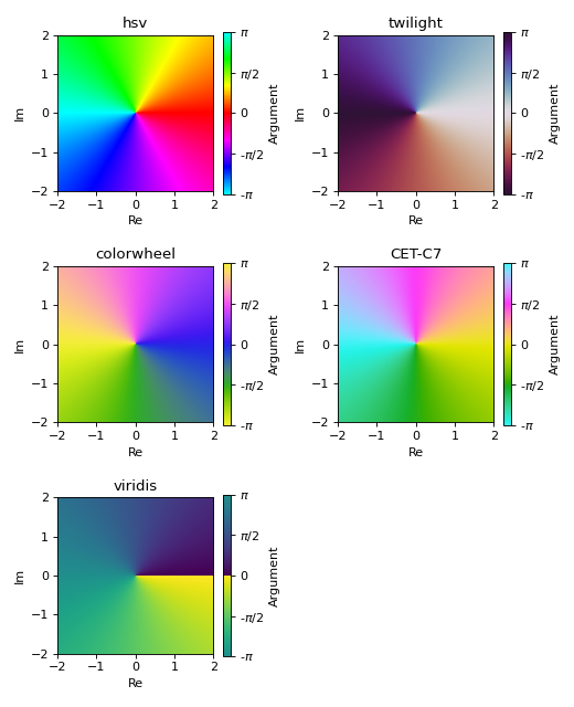
Hence, it might be helpful to chose a perceptually uniform colormap. Domaing coloring plots are naturally suited to be represented by cyclic colormaps, but sequential colormaps can be used too. In the following example we illustrate the phase portrait of f(z) = z using different colormaps:
from sympy import symbols, pi
import colorcet
from spb import *

z = symbols("z")
cmaps = {
    "hsv": "hsv",
    "twilight": "twilight",
    "colorwheel": colorcet.colorwheel,
    "CET-C7": colorcet.CET_C7,
    "viridis": "viridis"
}
plots = []
for k, v in cmaps.items():
    plots.append(
        plot_complex(z, (z, -2-2j, 2+2j), coloring="a",
            grid=False, show=False, legend=True, cmap=v, title=k))

plotgrid(*plots, nc=2, size=(6.5, 8))
(
Source code,png,hires.png,pdf)
In the above figure, when using the HSV colormap the eye is drawn to the yellow, cyan and magenta colors, where there is a lightness gradient: those are false features caused by the colormap. Indeed, there is nothing going on these regions when looking with a perceptually uniform colormap.
Phase is computed with Numpy and lies between [-pi, pi]. Then, phase is normalized between [0, 1] using (arg / (2 * pi)) % 1. The figure below shows the mapping between phase in radians and normalized phase. A phase of 0 radians corresponds to a normalized phase of 0, which gets mapped to the beginning of a colormap.
(
Source code,png,hires.png,pdf)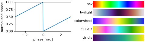
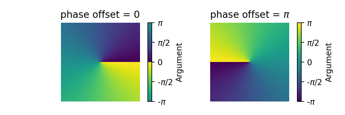
The zero radians phase is then located in the middle of the colorbar. Hence, the colorbar might feel “weird” if a sequential colormap is chosen, because there is a color-discontinuity in the middle of it, as can be seen in the previous example. The
phaseoffsetkeyword argument allows to adjust the position of the colormap:p1 = plot_complex( z, (z, -2-2j, 2+2j), grid=False, show=False, legend=True, coloring="a", cmap="viridis", phaseoffset=0, title="phase offset = 0", axis=False) p2 = plot_complex( z, (z, -2-2j, 2+2j), grid=False, show=False, legend=True, coloring="a", cmap="viridis", phaseoffset=pi, title=r"phase offset = $\pi$", axis=False) plotgrid(p1, p2, nc=2, size=(6, 2))
(
Source code,png,hires.png,pdf)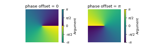
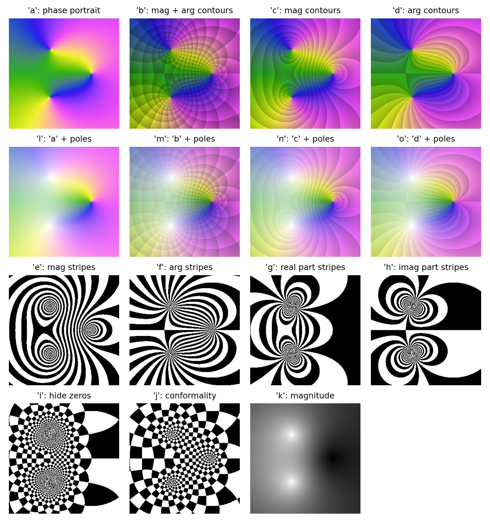
A pure phase portrait is rarely useful, as it conveys too little information. Let’s now quickly visualize the different
coloringschemes. In the following, arg is the argument (phase), mag is the magnitude (absolute value) and contour is a line of constant value. Refer to [1] for more information.from matplotlib import rcParams rcParams["font.size"] = 8 colorings = "abcdlmnoefghijk" titles = [ "phase portrait", "mag + arg contours", "mag contours", "arg contours", "'a' + poles", "'b' + poles", "'c' + poles", "'d' + poles", "mag stripes", "arg stripes", "real part stripes", "imag part stripes", "hide zeros", "conformality", "magnitude"] plots = [] expr = (z - 1) / (z**2 + z + 1) for c, t in zip(colorings, titles): plots.append( plot_complex(expr, (z, -2-2j, 2+2j), coloring=c, grid=False, show=False, legend=False, cmap=colorcet.CET_C2, axis=False, colorbar=False, title=("'%s'" % c) + ": " + t, xlabel="", ylabel="")) plotgrid(*plots, nc=4, size=(8, 8.5))
(
Source code,png,hires.png,pdf)
From the above picture, we can see that:
Some enhancements decrese the lighness of the colors: depending on the colormap, it might be difficult to distinguish features in darker regions.
Other enhancements increases the lightness in proximity of poles. Hence, colormaps with very light colors might not convey enough information.
With this considerations in mind, the selection of a proper colormap is left to the user because not only it depends on the target audience of the visualization, but also on the function being visualized.
References
Examples
>>> from sympy import I, symbols, exp, sqrt, cos, sin, pi, gamma
>>> from spb import plot_complex
>>> x, y, z = symbols('x, y, z')
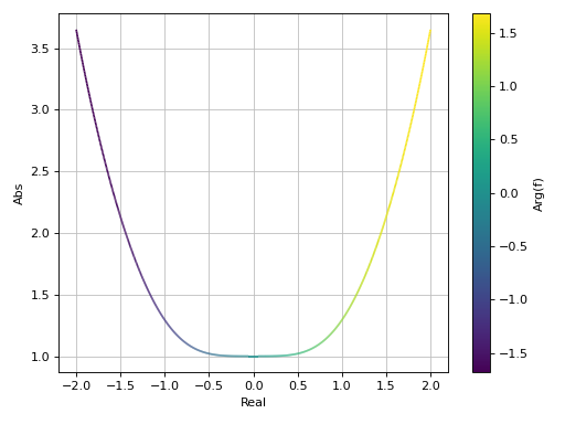
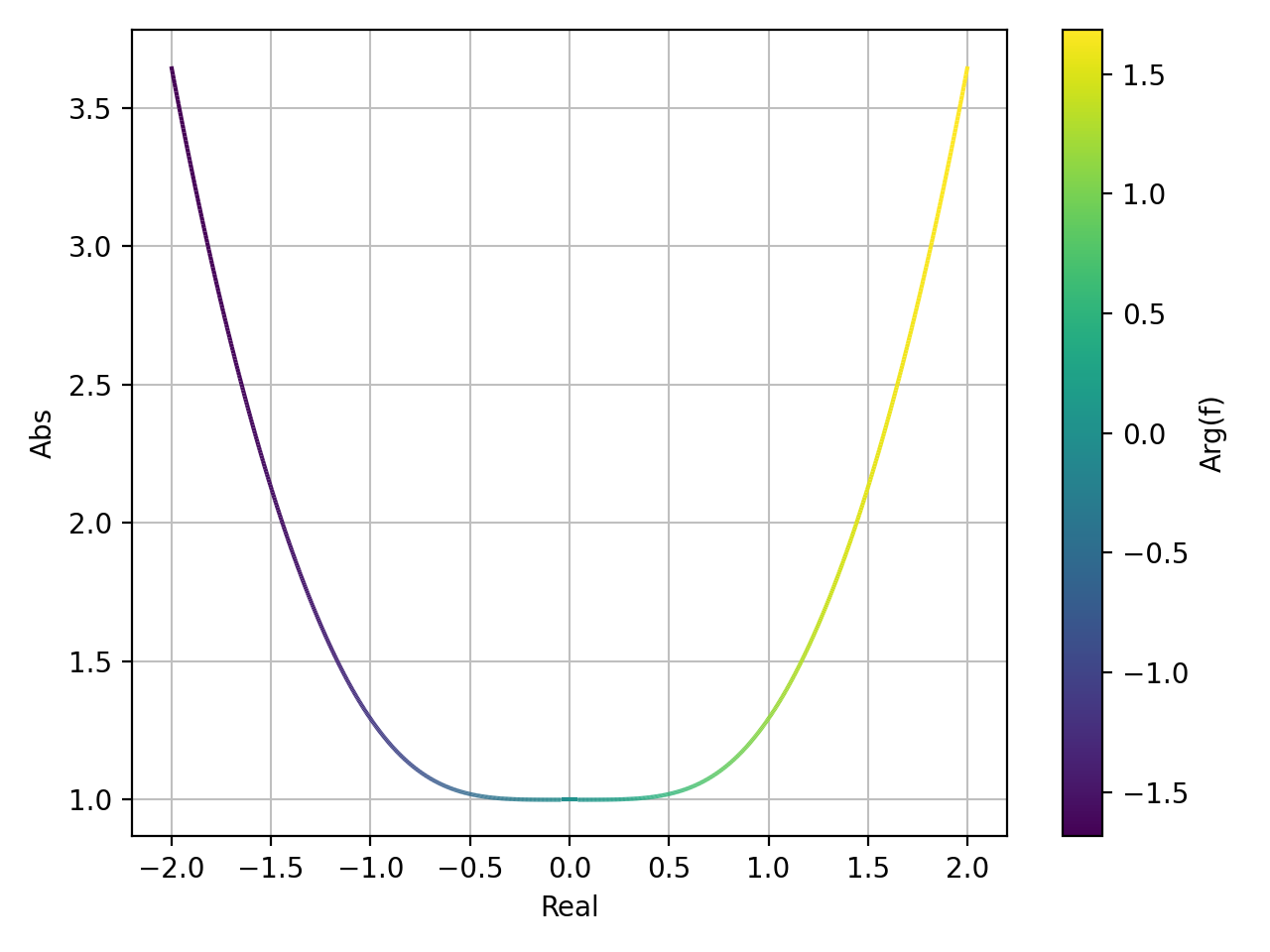
Plot the modulus of a complex function colored by its magnitude:
>>> plot_complex(cos(x) + sin(I * x), "f", (x, -2, 2))
Plot object containing:
[0]: cartesian abs-arg line: cos(x) + I*sinh(x) for x over ((-2+0j), (2+0j))
(
Source code,png,hires.png,pdf)
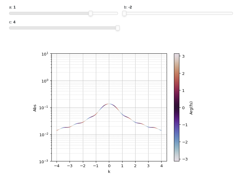
Interactive-widget plot of a Fourier Transform. Refer to the interactive sub-module documentation to learn more about the
paramsdictionary. This plot illustrates:the use of
prange(parametric plotting range).for
plot_complex, symbols going intoprangemust be real.the use of the
paramsdictionary to specify sliders in their basic form: (default, min, max).
from sympy import *
from spb import *
x, k, a, b = symbols("x, k, a, b")
c = symbols("c", real=True)
f = exp(-x**2) * (Heaviside(x + a) - Heaviside(x - b))
fs = fourier_transform(f, x, k)
plot_complex(fs, prange(k, -c, c),
        params={a: (1, -2, 2), b: (-2, -2, 2), c: (4, 0.5, 4)},
        label="Arg(fs)", xlabel="k", yscale="log", ylim=(1e-03, 10),
        use_latex=False)
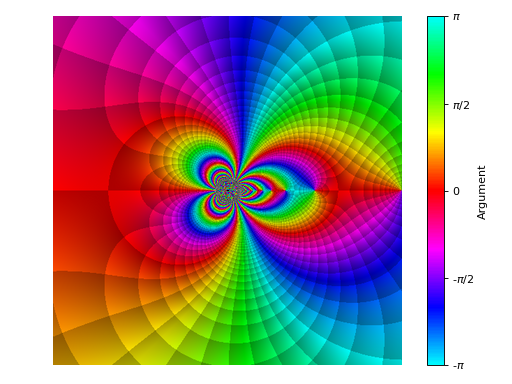
Domain coloring plot. To improve the smoothness of the results, increase the number of discretization points and/or apply an interpolation (if the backend supports it):
>>> plot_complex(gamma(z), (z, -3-3j, 3+3j),
...     coloring="b", n=500, grid=False)
Plot object containing:
[0]: complex domain coloring: gamma(z) for re(z) over (-3.0, 3.0) and im(z) over (-3.0, 3.0)
(
Source code,png,hires.png,pdf)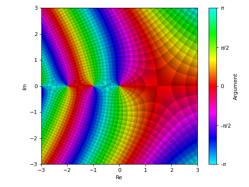
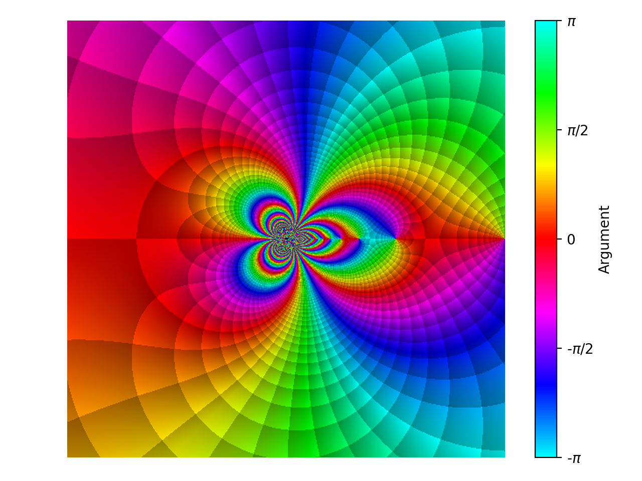
Domain coloring of the same function evaluated near the point \(z=\infty\):
>>> plot_complex(gamma(z), (z, -1-1j, 1+1j), coloring="b", n=500,
...     grid=False, at_infinity=True, axis=False)
Plot object containing:
[0]: complex domain coloring: gamma(1/z) for re(z) over (-1.0, 1.0) and im(z) over (-1.0, 1.0)
(
Source code,png,hires.png,pdf)
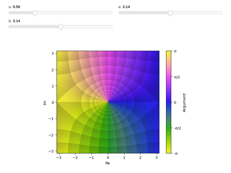
Interactive-widget domain coloring plot. Refer to the interactive sub-module documentation to learn more about the
paramsdictionary. This plot illustrates:setting a custom colormap and adjusting the black-level of the enhanced visualization.
the use of
prange(parametric plotting range).the use of the
paramsdictionary to specify sliders in their basic form: (default, min, max).
from sympy import *
from spb import *
import colorcet
z, u, a, b = symbols("z, u, a, b")
plot_complex(
    sin(u * z), prange(z, -a - b*I, a + b*I),
    cmap=colorcet.colorwheel, blevel=0.85, use_latex=False,
    coloring="b", n=250, grid=False,
    params={
        u: (0.5, 0, 2),
        a: (pi, 0, 2*pi),
        b: (pi, 0, 2*pi),
    })

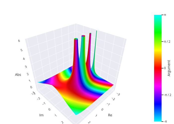
The analytic landscape is 3D plot of the absolute value of a complex function colored by its argument:
from sympy import symbols, gamma, I
from spb import plot_complex, PB
z = symbols('z')
plot_complex(gamma(z), (z, -3 - 3*I, 3 + 3*I), threed=True,
    backend=PB, zlim=(-1, 6), use_cm=True)
(Source code, png, pdf, html)
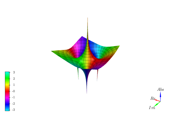
Because the function goes to infinity at poles, sometimes it might be beneficial to visualize the logarithm of the absolute value in order to easily identify zeros:
from sympy import symbols, I
from spb import plot_complex, KB
z = symbols("z")
expr = (z**3 - 5) / z
plot_complex(expr, (z, -3-3j, 3+3j), coloring="b", threed=True,
    use_cm=True, grid=False, n=500, backend=KB, tz=np.log)

- spb.ccomplex.complex.plot_riemann_sphere(*args, **kwargs)[source]
Visualize stereographic projections of the Riemann sphere.
Note:
Differently from other plot functions that return instances of
BaseBackend, this function returns a Matplotlib figure.This function calls
plot_complex: refer to its documentation for the full list of keyword arguments.
- Parameters:
- args
- exprExpr
Represent the complex function to be plotted.
- range3-element tuple, optional
Denotes the range of the variables. Only works for 2D plots. Default to
(z, -1.25 - 1.25*I, 1.25 + 1.25*I).
- annotateboolean, optional
Turn on/off the annotations on the 2D projections of the Riemann sphere. Default to True (annotations are visible). They can only be visible when
riemann_mask=True.- riemann_maskboolean, optional
Turn on/off the unit disk mask representing the Riemann sphere on the 2D projections. Default to True (mask is active).
- axisboolean, optional
Turn on/off the axis of the 2D subplots. Default to False (axis not visible).
- size(width, height)
Specify the size of the resulting figure.
- titlestr, list, optional
A list of two strings representing the titles for the two plots.
See also
Notes
The Riemann sphere[#fn5]_ is a model of the extented complex plane, comprised of the complex plane plus a point at infinity. Let’s consider a 3D space with a sphere of radius 1 centered at the origin. The xy plane, representing the complex plane, cut the sphere in half at the equator. The stereographic projection of any point in the complex plane on the sphere is given by the intersection point between a line connecting the complex point with the north pole of the sphere. Let’s consider the magnitude of a complex point:
if its lower than one (points inside the unit disk), then the point is mapped to the Southern Hemisphere (the line connecting the complex point to the north pole intersects the sphere in the Southern Hemisphere). The origin of the complex plane is mapped to the south pole.
if its equal to one (points in the unit circle), then the point is already on the sphere, specifically in its equator.
if its greater than one (point outside the unit disk), then the point is mapped to the Northen Hemisphere. The north pole represents the point at infinity.
Visualizing a 3D sphere is difficult (refer to Wegert [4] for more information): the most obvious problem is that only a part can be seen from any location. A better way to fully visualize the sphere is with two 2D charts depicting the sphere from the inside:
a stereographic projection of the sphere from the north pole, which depict the Southern Hemisphere. It corresponds to an ordinary (enhanced) domain coloring plot around the complex point \(z=0\).
a stereographic projection of the sphere from the south pole, which depict the Northen Hemisphere. It corresponds to an ordinary (enhanced) domain coloring plot around the complex point \(z=\infty\) (infinity). Practically, it depicts the transformation \(z \rightarrow \frac{1}{z}\).
Let’s look at an example:
from sympy import symbols, pi
from spb import *
z = symbols("z")
expr = (z - 1) / (z**2 + z + 2)
plot_riemann_sphere(expr, coloring="b", n=800)
(
Source code,png,hires.png,pdf)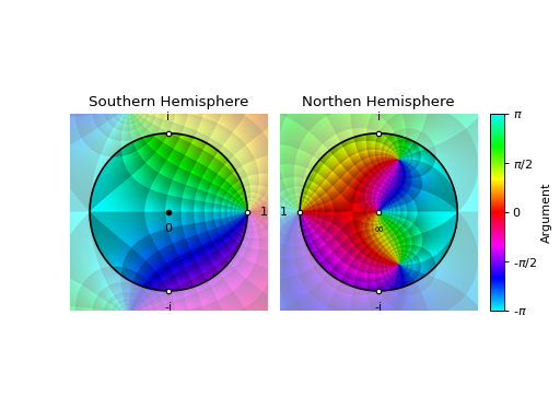
The saturated disks represents the hemispheres. The black circle is the equator. Also, a few important points are displayed to make the plot easier to understand.
Note the orientation of the Northen Hemisphere: it has been rotated around the point at infinity by an angle pi and flipped about the real axis. This is convenient because:
we can now imagine to fold the two charts so that the points 1, i, -i are overlayed, glue the equator and blow it up to obtain a sphere.
imagine bringing the two discs closer so that they touch at the point 1. Now, roll the two discs together: assuming there are no branch cuts, there is continuity of argument and absolute value across the equator: what is outside of the disc in the left plot, is inside of the disk in the second plot, and vice-versa.
From the above plots, the zero located at \(z=1\) is clearly visible, as well as the two poles located at \(z = -\frac{1}{2} - i \frac{\sqrt{7}}{2}\) and \(z = -\frac{1}{2} + i \frac{\sqrt{7}}{2}\). Not obvious at first, there is a zero located at \(z=\infty\). We can tell its a zero by looking at ordering of colors around it in comparison to the poles. Alternatively, we can use some enhanced color scheme, for example one which brings poles to white:
plot_riemann_sphere(expr, coloring="m", n=800)
(
Source code,png,hires.png,pdf)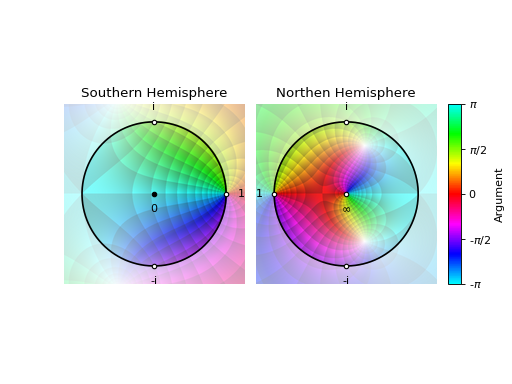
References
Examples
Standard output:
from sympy import symbols, Rational, I
from spb import *
z = symbols("z")
expr = 1 / (2 * z**2) + z
plot_riemann_sphere(expr, coloring="b", n=800)
(
Source code,png,hires.png,pdf)
Hide annotations:
plot_riemann_sphere(expr, coloring="b", n=800, annotate=False)
(
Source code,png,hires.png,pdf)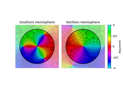
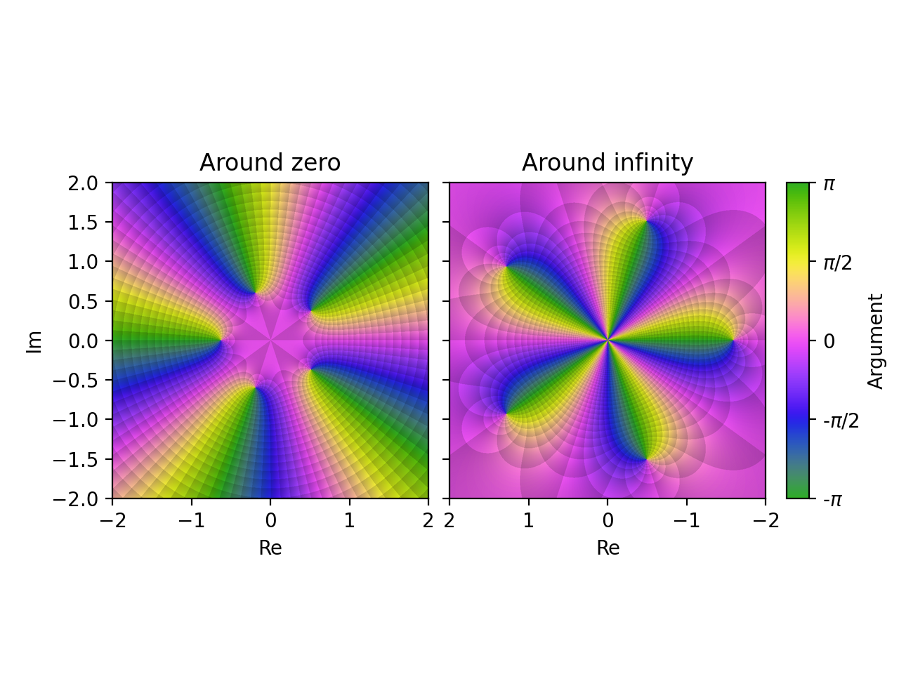
Hiding Riemann disk mask and annotations, set a custom domain, show axis (note that the right-most plot might be misleading because the center represents infinity), custom colormap, set the black level of contours, set titles.
import colorcet
expr = z**5 + Rational(1, 10)
l = 2
plot_riemann_sphere(
    expr, (z, -l-l*I, l+l*I), coloring="b", n=800,
    riemann_mask=False, axis=True, grid=False,
    cmap=colorcet.CET_C2, blevel=0.85,
    title=["Around zero", "Around infinity"])
(
Source code,png,hires.png,pdf)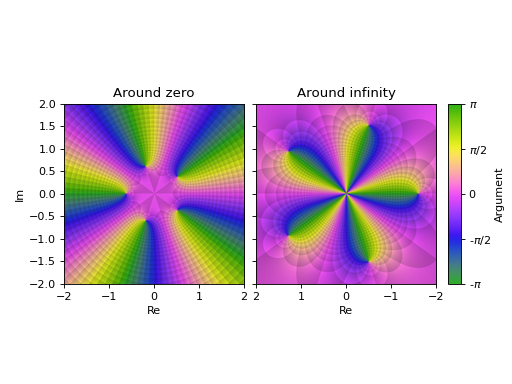
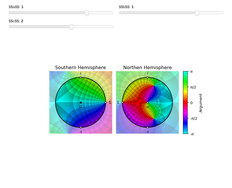
Interactive-widget plot. Refer to the interactive sub-module documentation to learn more about the
paramsdictionary. This plot illustrates the use of theparamsdictionary to specify sliders in their basic form: (default, min, max).from sympy import * from sympy.abc import a, b, c from spb import * z = symbols("z") expr = (z - 1) / (a * z**2 + b * z + c) plot_riemann_sphere( expr, coloring="b", n=300, params={ a: (1, -2, 2), b: (1, -2, 2), c: (2, -10, 10), }, use_latex=False )
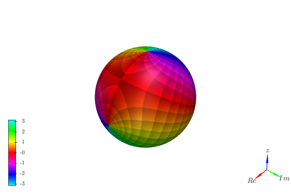
3D plot of a complex function on the Riemann sphere. Note, the higher the number of discretization points, the better the final results, but the higher memory consumption:
from sympy import *
from spb import *
z = symbols("z")
expr = (z - 1) / (z**2 + z + 1)
plot_riemann_sphere(expr, threed=True, n=150,
    coloring="b", backend=KB, legend=False, grid=False)

- spb.ccomplex.complex.plot_complex_list(*args, **kwargs)[source]
Plot lists of complex points. By default, the aspect ratio of the plot is set to
aspect="equal".Typical usage examples are in the followings:
- Plotting a single list of complex numbers.
plot_complex_list(l1, **kwargs)
- Plotting multiple lists of complex numbers.
plot_complex_list(l1, l2, **kwargs)
- Plotting multiple lists of complex numbers each one with a custom label.
plot_complex_list((l1, label1), (l2, label2), **kwargs)
- Parameters:
- args
- numberslist, tuple
A list of complex numbers.
- labelstr
The name associated to the list of the complex numbers to be eventually shown on the legend. Default to empty string.
- rendering_kwdict, optional
A dictionary of keywords/values which is passed to the backend’s function to customize the appearance of lines. Refer to the plotting library (backend) manual for more informations. Note that the same options will be applied to all series generated for the specified expression.
- aspect(float, float) or str, optional
Set the aspect ratio of the plot. The value depends on the backend being used. Read that backend’s documentation to find out the possible values.
- backendPlot, optional
A subclass of
Plot, which will perform the rendering. Default toMatplotlibBackend.- is_pointboolean
If True, a scatter plot will be produced. Otherwise a line plot will be created. Default to True.
- is_filledboolean, optional
Default to True, which will render empty circular markers. It only works if
is_point=True. If False, filled circular markers will be rendered.- labelstr or list/tuple, optional
The name associated to the list of the complex numbers to be eventually shown on the legend. The number of labels must be equal to the number of series generated by the plotting function.
- paramsdict
A dictionary mapping symbols to parameters. This keyword argument enables the interactive-widgets plot, which doesn’t support the adaptive algorithm (meaning it will use
adaptive=False). Learn more by reading the documentation of the interactive sub-module.- rendering_kwdict or list of dicts, optional
A dictionary of keywords/values which is passed to the backend’s function to customize the appearance of lines. Refer to the plotting library (backend) manual for more informations. If a list of dictionaries is provided, the number of dictionaries must be equal to the number of series generated by the plotting function.
- showboolean
Default to True, in which case the plot will be shown on the screen.
- size(float, float), optional
A tuple in the form (width, height) to specify the size of the overall figure. The default value is set to None, meaning the size will be set by the backend.
- titlestr, optional
Title of the plot. It is set to the latex representation of the expression, if the plot has only one expression.
- use_latexboolean, optional
Turn on/off the rendering of latex labels. If the backend doesn’t support latex, it will render the string representations instead.
- xlabel, ylabelstr, optional
Labels for the x-axis or y-axis, respectively.
- xscale, yscale‘linear’ or ‘log’, optional
Sets the scaling of the x-axis or y-axis, respectively. Default to
'linear'.- xlim, ylim(float, float), optional
Denotes the x-axis limits or y-axis limits, respectively,
(min, max).
See also
Examples
>>> from sympy import I, symbols, exp, sqrt, cos, sin, pi, gamma
>>> from spb import plot_complex_list
>>> x, y, z = symbols('x, y, z')
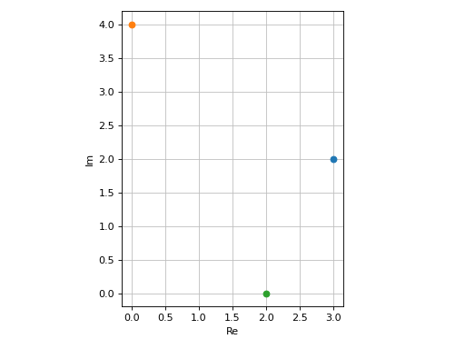
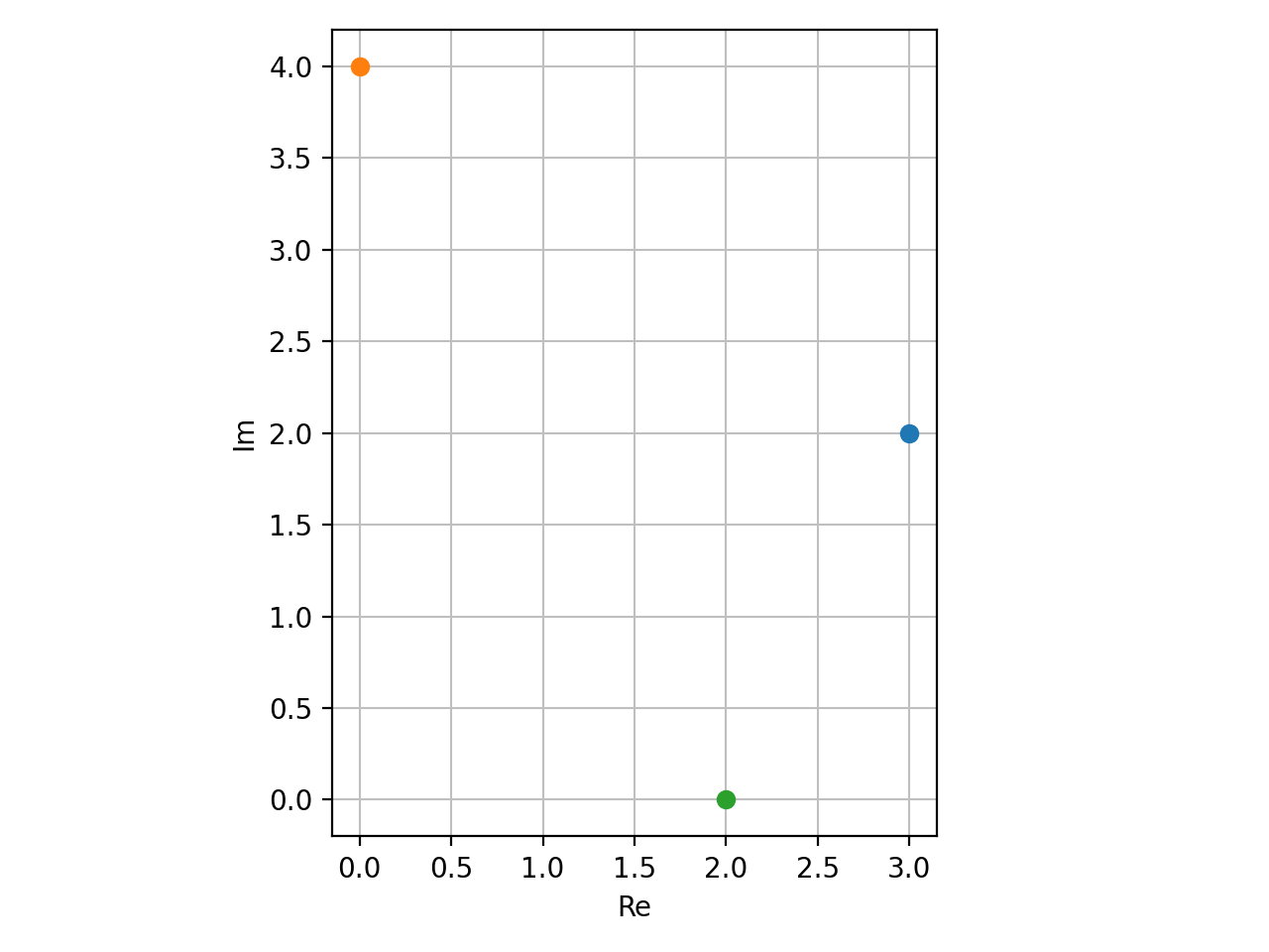
Plot individual complex points:
>>> plot_complex_list(3 + 2 * I, 4 * I, 2)
Plot object containing:
[0]: complex points: (3 + 2*I,)
[1]: complex points: (4*I,)
[2]: complex points: (2,)
(
Source code,png,hires.png,pdf)
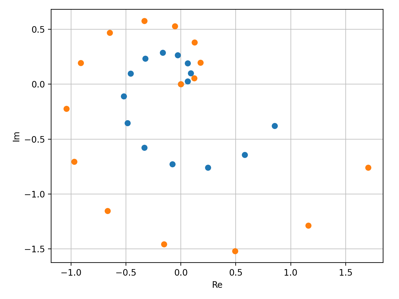
Plot two lists of complex points and assign to them custom labels:
>>> expr1 = z * exp(2 * pi * I * z)
>>> expr2 = 2 * expr1
>>> n = 15
>>> l1 = [expr1.subs(z, t / n) for t in range(n)]
>>> l2 = [expr2.subs(z, t / n) for t in range(n)]
>>> plot_complex_list((l1, "f1"), (l2, "f2"))
Plot object containing:
[0]: complex points: (0.0, 0.0666666666666667*exp(0.133333333333333*I*pi), 0.133333333333333*exp(0.266666666666667*I*pi), 0.2*exp(0.4*I*pi), 0.266666666666667*exp(0.533333333333333*I*pi), 0.333333333333333*exp(0.666666666666667*I*pi), 0.4*exp(0.8*I*pi), 0.466666666666667*exp(0.933333333333333*I*pi), 0.533333333333333*exp(1.06666666666667*I*pi), 0.6*exp(1.2*I*pi), 0.666666666666667*exp(1.33333333333333*I*pi), 0.733333333333333*exp(1.46666666666667*I*pi), 0.8*exp(1.6*I*pi), 0.866666666666667*exp(1.73333333333333*I*pi), 0.933333333333333*exp(1.86666666666667*I*pi))
[1]: complex points: (0, 0.133333333333333*exp(0.133333333333333*I*pi), 0.266666666666667*exp(0.266666666666667*I*pi), 0.4*exp(0.4*I*pi), 0.533333333333333*exp(0.533333333333333*I*pi), 0.666666666666667*exp(0.666666666666667*I*pi), 0.8*exp(0.8*I*pi), 0.933333333333333*exp(0.933333333333333*I*pi), 1.06666666666667*exp(1.06666666666667*I*pi), 1.2*exp(1.2*I*pi), 1.33333333333333*exp(1.33333333333333*I*pi), 1.46666666666667*exp(1.46666666666667*I*pi), 1.6*exp(1.6*I*pi), 1.73333333333333*exp(1.73333333333333*I*pi), 1.86666666666667*exp(1.86666666666667*I*pi))
(
Source code,png,hires.png,pdf)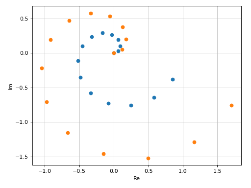
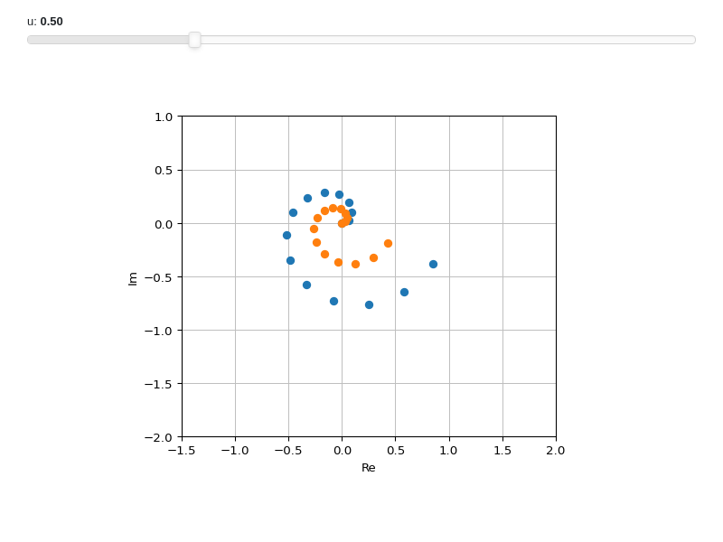
Interactive-widget plot. Refer to the interactive sub-module documentation to learn more about the
paramsdictionary.from sympy import * from spb import * z, u = symbols("z u") expr1 = z * exp(2 * pi * I * z) expr2 = u * expr1 n = 15 l1 = [expr1.subs(z, t / n) for t in range(n)] l2 = [expr2.subs(z, t / n) for t in range(n)] plot_complex_list( (l1, "f1"), (l2, "f2"), params={u: (0.5, 0, 2)}, use_latex=False, xlim=(-1.5, 2), ylim=(-2, 1))

- spb.ccomplex.complex.plot_real_imag(*args, **kwargs)[source]
Plot the real part, the imaginary parts, the absolute value and the argument of a complex function. By default, only the real and imaginary parts will be plotted. Use keyword argument to be more specific. By default, the aspect ratio of 2D plots is set to
aspect="equal".Depending on the provided expression, this function will produce different types of plots:
line plot over the reals.
surface plot over the complex plane if threed=True.
contour plot over the complex plane if threed=False.
Typical usage examples are in the followings:
- Plotting a single expression with a single range.
plot_real_imag(expr, range, **kwargs)
- Plotting a single expression with the default range (-10, 10).
plot_real_imag(expr, **kwargs)
- Plotting multiple expressions with a single range.
plot_real_imag(expr1, expr2, …, range, **kwargs)
- Plotting multiple expressions with multiple ranges.
plot_real_imag((expr1, range1), (expr2, range2), …, **kwargs)
- Plotting multiple expressions with custom labels and rendering options.
plot_real_imag((expr1, range1, label1, rendering_kw1), (expr2, range2, label2, rendering_kw2), …, **kwargs)
- Parameters:
- args
- exprExpr
Represent the complex function to be plotted.
- range3-element tuple
Denotes the range of the variables. For example:
(z, -5, 5): plot a line over the reals from point -5 to 5(z, -5 + 2*I, 5 + 2*I): plot a line from complex point(-5 + 2*I)to(5 + 2 * I). Note the same imaginary part for the start/end point. Also note that we can specify the ranges by using standard Python complex numbers, for example(z, -5+2j, 5+2j).(z, -5 - 3*I, 5 + 3*I): surface or contour plot of the complex function over the specified domain using a rectangular discretization.
- labelstr, optional
The name of the complex function to be eventually shown on the legend. If none is provided, the string representation of the function will be used.
- rendering_kwdict, optional
A dictionary of keywords/values which is passed to the backend’s function to customize the appearance of lines. Refer to the plotting library (backend) manual for more informations. Note that the same options will be applied to all series generated for the specified expression.
- absboolean, optional
If True, plot the modulus of the complex function. Default to False.
- adaptivebool, optional
If
True, creates line plots by using an adaptive algorithm. Useadaptive_goalandloss_fnto further customize the output. Image and surface plots do not use an adaptive algorithm.Default to
False, which uses a uniform sampling strategy.- adaptive_goalcallable, int, float or None
Controls the “smoothness” of the evaluation. Possible values:
None(default): it will use the following goal:lambda l: l.loss() < 0.01number (int or float). The lower the number, the more evaluation points. This number will be used in the following goal:
lambda l: l.loss() < numbercallable: a function requiring one input element, the learner. It must return a float number. Refer to [7] for more information.
- argboolean, optional
If True, plot the argument of the complex function. Default to False.
- aspect(float, float) or str, optional
Set the aspect ratio of the plot. The value depends on the backend being used. Read that backend’s documentation to find out the possible values.
- backendPlot, optional
A subclass of
Plot, which will perform the rendering. Default toMatplotlibBackend.- colorbarboolean, optional
Show/hide the colorbar. Only works when
use_cm=Trueand 3D plots. Default to True (colorbar is visible).- detect_polesboolean, optional
Chose whether to detect and correctly plot poles. Defaulto to False. It only works with line plots. To improve detection, increase the number of discretization points if
adaptive=Falseand/or change the value ofeps.- epsfloat, optional
An arbitrary small value used by the
detect_polesalgorithm. Default value to 0.1. Before changing this value, it is better to increase the number of discretization points.- imagboolean, optional
If True, plot the imaginary part of the complex function. Default to True.
- labellist/tuple, optional
The labels to be shown in the legend. If not provided, the string representation of
exprwill be used. The number of labels must be equal to the number of series generated by the plotting function.- loss_fncallable or None
The loss function to be used by the adaptive learner. Possible values:
None(default): it will use thedefault_lossfrom theadaptivemodule.callable : Refer to [7] for more information. Specifically, look at
adaptive.learner.learner1Dto find more loss functions.
- modulesstr, optional
Specify the modules to be used for the numerical evaluation. Refer to
lambdifyto visualize the available options. Default to None, meaning Numpy/Scipy will be used. Note that other modules might produce different results, based on the way they deal with branch cuts.- n1, n2int, optional
Number of discretization points in the real/imaginary-directions, respectively, when adaptive=False. For line plots, default to 1000. For surface/contour plots (2D and 3D), default to 300.
- nint or two-elements tuple (n1, n2), optional
If an integer is provided, set the same number of discretization points in all directions. If a tuple is provided, it overrides
n1andn2. It only works whenadaptive=False.- paramsdict
A dictionary mapping symbols to parameters. This keyword argument enables the interactive-widgets plot, which doesn’t support the adaptive algorithm (meaning it will use
adaptive=False). Learn more by reading the documentation of the interactive sub-module.- rendering_kwdict or list of dicts, optional
A dictionary of keywords/values which is passed to the backend’s function to customize the appearance of lines. Refer to the plotting library (backend) manual for more informations. If a list of dictionaries is provided, the number of dictionaries must be equal to the number of series generated by the plotting function.
- realboolean, optional
If True, plot the real part of the complex function. Default to True.
- showboolean, optional
Default to True, in which case the plot will be shown on the screen.
- size(float, float), optional
A tuple in the form (width, height) to specify the size of the overall figure. The default value is set to None, meaning the size will be set by the backend.
- surface_kwdict, optional
A dictionary of keywords/values which is passed to the backend’s function to customize the appearance of surfaces. Refer to the plotting library (backend) manual for more informations.
- threedboolean, optional
It only applies to a complex function over a complex range. If False, contour plots will be shown. If True, 3D surfaces will be shown. Default to False.
- use_cmboolean, optional
If False, surfaces will be rendered with a solid color. If True, a color map highlighting the elevation will be used. Default to True.
- use_latexboolean, optional
Turn on/off the rendering of latex labels. If the backend doesn’t support latex, it will render the string representations instead.
- titlestr, optional
Title of the plot. It is set to the latex representation of the expression, if the plot has only one expression.
- wireframeboolean, optional
Enable or disable a wireframe over the 3D surface. Depending on the number of wireframe lines (see
wf_n1andwf_n2), activating thisoption might add a considerable overhead during the plot’s creation. Default to False (disabled).- wf_n1, wf_n2int, optional
Number of wireframe lines along the x and y ranges, respectively. Default to 10. Note that increasing this number might considerably slow down the plot’s creation.
- wf_npointint or None, optional
Number of discretization points for the wireframe lines. Default to None, meaning that each wireframe line will have
n1orn2number of points, depending on the line direction.- wf_rendering_kwdict, optional
A dictionary of keywords/values which is passed to the backend’s function to customize the appearance of wireframe lines.
- xlabel, ylabel, zlabelstr, optional
Labels for the x-axis, y-axis or z-axis, respectively.
zlabelis only available for 3D plots.- xscale, yscale‘linear’ or ‘log’, optional
Sets the scaling of the x-axis or y-axis, respectively. Default to
'linear'.- xlim, ylim, zlim(float, float), optional
Denotes the x-axis limits, y-axis limits or z-axis limits, respectively,
(min, max).zlimis only available for 3D plots.
See also
References
Examples
>>> from sympy import I, symbols, exp, sqrt, cos, sin, pi, gamma
>>> from spb import plot_real_imag
>>> x, y, z = symbols('x, y, z')
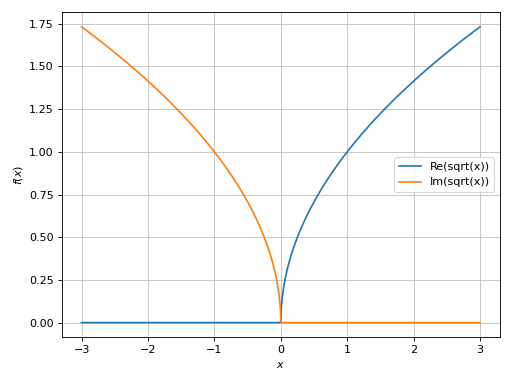
Plot the real and imaginary parts of a function over reals:
>>> plot_real_imag(sqrt(x), (x, -3, 3))
Plot object containing:
[0]: cartesian line: re(sqrt(x)) for x over (-3.0, 3.0)
[1]: cartesian line: im(sqrt(x)) for x over (-3.0, 3.0)
(
Source code,png,hires.png,pdf)
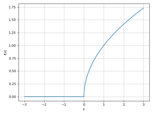
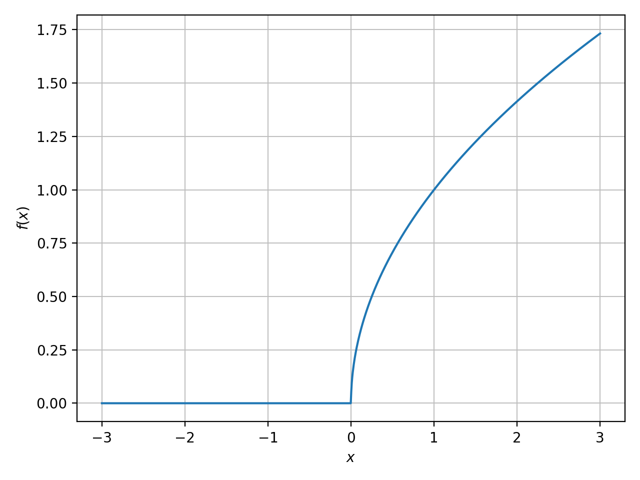
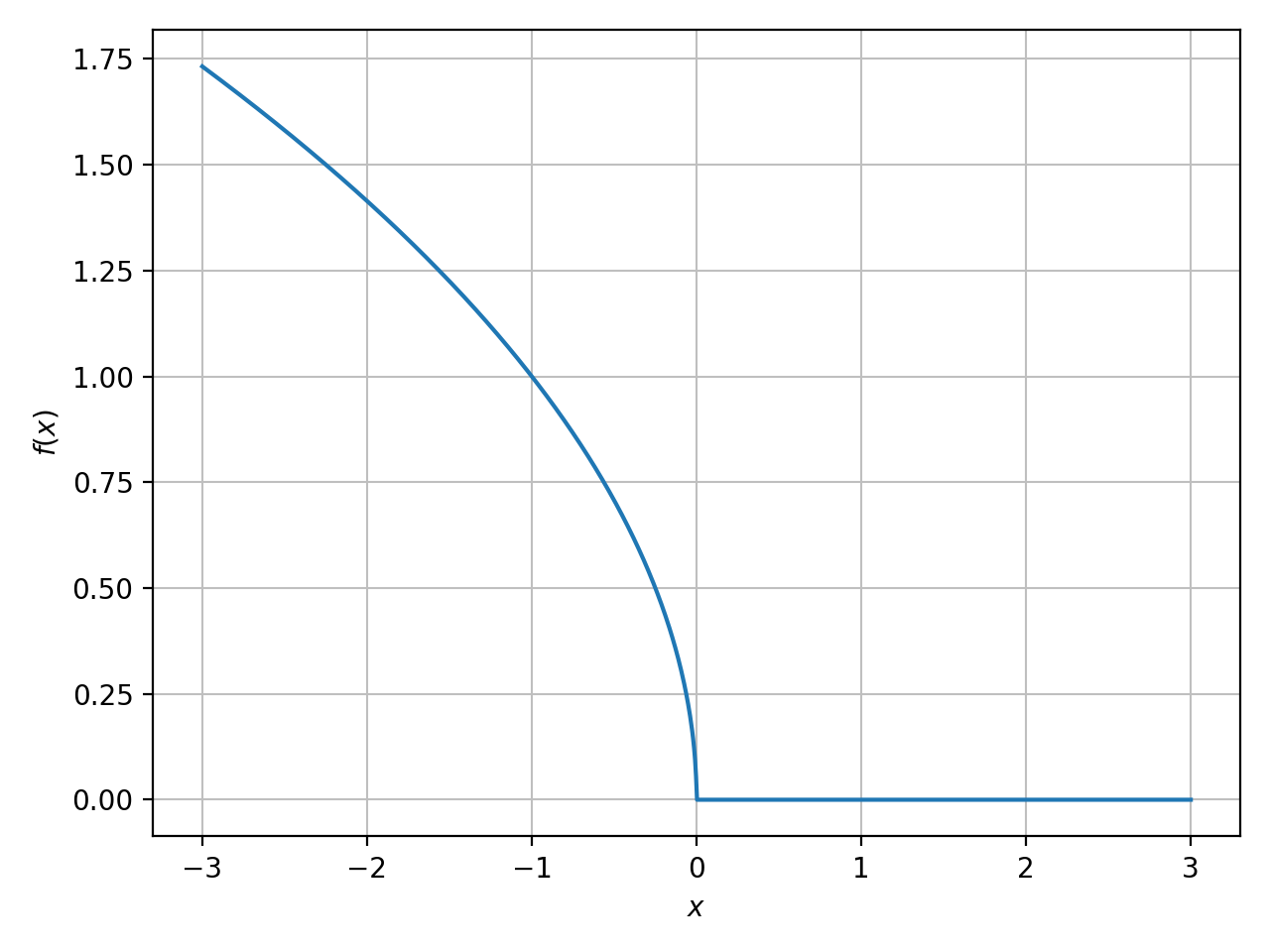
Plot only the real part:
>>> plot_real_imag(sqrt(x), (x, -3, 3), imag=False)
Plot object containing:
[0]: cartesian line: re(sqrt(x)) for x over (-3.0, 3.0)
(
Source code,png,hires.png,pdf)
Plot only the imaginary part:
>>> plot_real_imag(sqrt(x), (x, -3, 3), real=False)
Plot object containing:
[0]: cartesian line: im(sqrt(x)) for x over (-3.0, 3.0)
(
Source code,png,hires.png,pdf)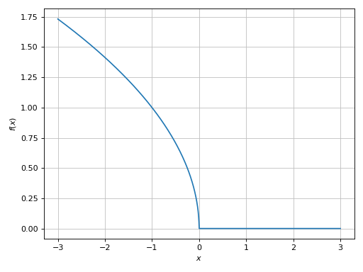
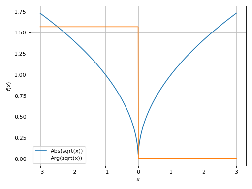
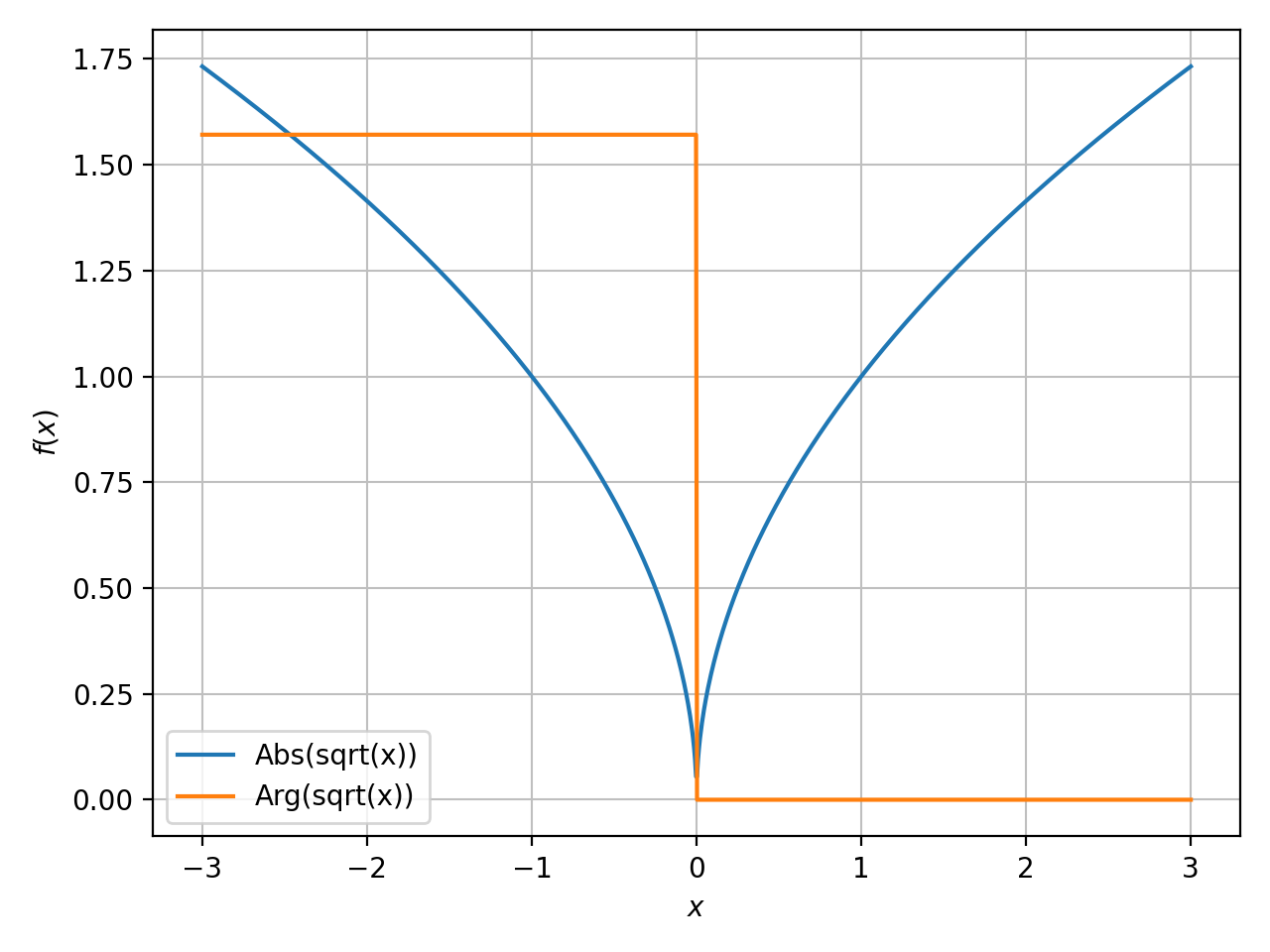
Plot only the absolute value and argument:
>>> plot_real_imag(sqrt(x), (x, -3, 3), real=False, imag=False, abs=True, arg=True)
Plot object containing:
[0]: cartesian line: abs(sqrt(x)) for x over (-3.0, 3.0)
[1]: cartesian line: arg(sqrt(x)) for x over (-3.0, 3.0)
(
Source code,png,hires.png,pdf)
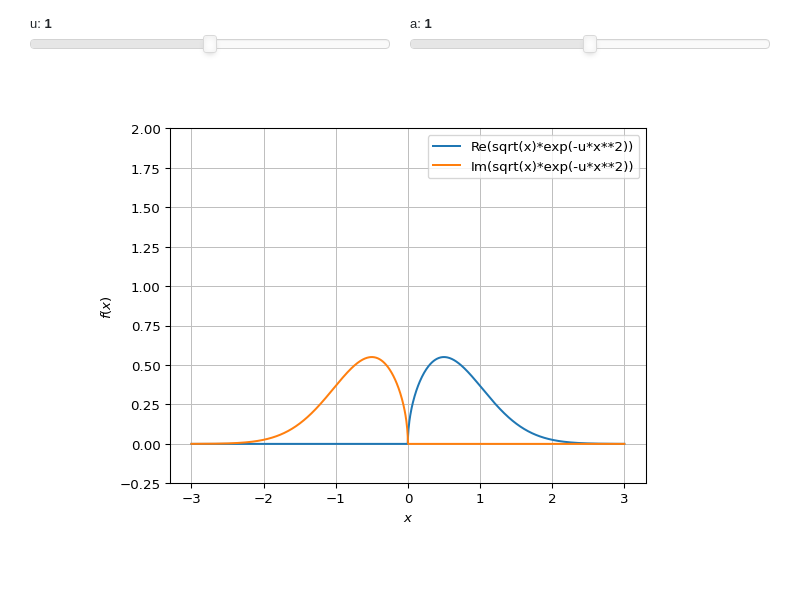
Interactive-widget plot. Refer to the interactive sub-module documentation to learn more about the
paramsdictionary. This plot illustrates:the use of
prange(parametric plotting range).for 1D
plot_real_imag, symbols going intoprangemust be real.the use of the
paramsdictionary to specify sliders in their basic form: (default, min, max).
from sympy import *
from spb import *
x, u = symbols("x, u")
a = symbols("a", real=True)
plot_real_imag(sqrt(x) * exp(-u * x**2), prange(x, -3*a, 3*a),
    params={u: (1, 0, 2), a: (1, 0, 2)},
    ylim=(-0.25, 2), use_latex=False)

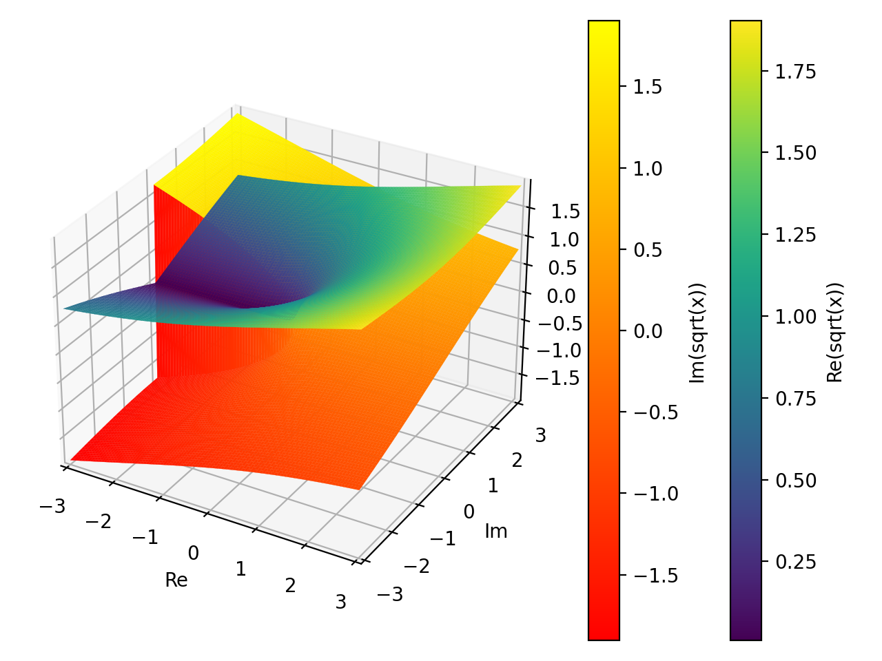
3D plot of the real and imaginary part of the principal branch of a function over a complex range. Note the jump in the imaginary part: that’s a branch cut. The rectangular discretization is unable to properly capture it, hence the near vertical wall. Refer to
plot3d_parametric_surfacefor an example about plotting Riemann surfaces and properly capture the branch cuts.>>> plot_real_imag(sqrt(x), (x, -3-3j, 3+3j), n=100, threed=True, ... use_cm=True) Plot object containing: [0]: complex cartesian surface: re(sqrt(x)) for re(x) over (-3.0, 3.0) and im(x) over (-3.0, 3.0) [1]: complex cartesian surface: im(sqrt(x)) for re(x) over (-3.0, 3.0) and im(x) over (-3.0, 3.0)
(
Source code,png,hires.png,pdf)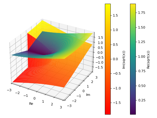
3D plot of the absolute value of a function over a complex range:
>>> plot_real_imag(sqrt(x), (x, -3-3j, 3+3j),
...     n=100, real=False, imag=False, abs=True, threed=True)
Plot object containing:
[0]: complex cartesian surface: abs(sqrt(x)) for re(x) over (-3.0, 3.0) and im(x) over (-3.0, 3.0)
(
Source code,png,hires.png,pdf)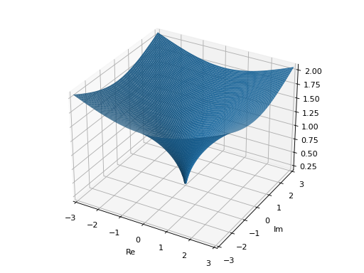
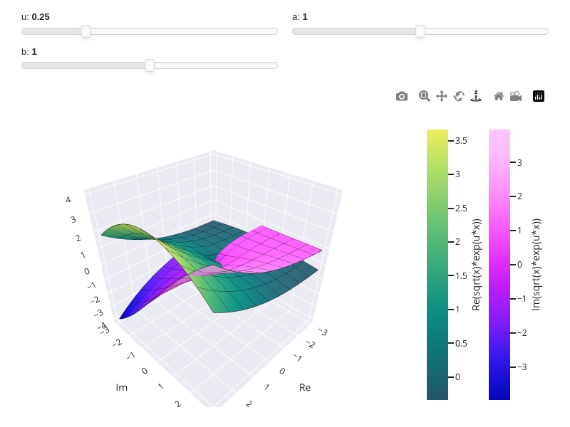
Interactive-widget plot. Refer to the interactive sub-module documentation to learn more about the
paramsdictionary. This plot illustrates:the use of
prange(parametric plotting range).the use of the
paramsdictionary to specify sliders in their basic form: (default, min, max).
from sympy import *
from spb import *
x, u, a, b = symbols("x, u, a, b")
plot_real_imag(
    sqrt(x) * exp(u * x), prange(x, -3*a-b*3j, 3*a+b*3j),
    backend=PB, aspect="cube",
    wireframe=True, wf_rendering_kw={"line_width": 1},
    params={
        u: (0.25, 0, 1),
        a: (1, 0, 2),
        b: (1, 0, 2)
    }, n=25, threed=True, use_latex=False, use_cm=True)

- spb.ccomplex.complex.plot_complex_vector(*args, **kwargs)[source]
Plot the vector field [re(f), im(f)] for a complex function f over the specified complex domain. By default, the aspect ratio of 2D plots is set to
aspect="equal".Typical usage examples are in the followings:
- Plotting a vector field of a complex function.
plot_complex_vector(expr, range, **kwargs)
- Plotting multiple vector fields with different ranges and custom labels.
plot_complex_vector((expr1, range1, label1 [optional]), (expr2, range2, label2 [optional]), **kwargs)
- Parameters:
- args
- exprExpr
Represent the complex function.
- range3-element tuples
Denotes the range of the variables. For example
(z, -5 - 3*I, 5 + 3*I). Note that we can specify the range by using standard Python complex numbers, for example(z, -5-3j, 5+3j).- labelstr, optional
The name of the complex expression to be eventually shown on the legend. If none is provided, the string representation of the expression will be used.
- aspect(float, float) or str, optional
Set the aspect ratio of the plot. The value depends on the backend being used. Read that backend’s documentation to find out the possible values.
- backendPlot, optional
A subclass of Plot, which will perform the rendering. Default to MatplotlibBackend.
- colorbarboolean, optional
Show/hide the colorbar. Default to True (colorbar is visible).
- contours_kwdict
A dictionary of keywords/values which is passed to the backend contour function to customize the appearance. Refer to the plotting library (backend) manual for more informations.
- n1, n2int
Number of discretization points for the quivers or streamlines in the x/y-direction, respectively. Default to 25.
- nint or two-elements tuple (n1, n2), optional
If an integer is provided, set the same number of discretization points in all directions for quivers or streamlines. If a tuple is provided, it overrides
n1andn2. It only works whenadaptive=False. Default to 25.- ncint
Number of discretization points for the scalar contour plot. Default to 100.
- paramsdict
A dictionary mapping symbols to parameters. This keyword argument enables the interactive-widgets plot, which doesn’t support the adaptive algorithm (meaning it will use
adaptive=False). Learn more by reading the documentation of the interactive sub-module.- quiver_kwdict
A dictionary of keywords/values which is passed to the backend quivers-plotting function to customize the appearance. Refer to the plotting library (backend) manual for more informations.
- scalarboolean, Expr, None or list/tuple of 2 elements
Represents the scalar field to be plotted in the background of a 2D vector field plot. Can be:
True: plot the magnitude of the vector field. Only works when a single vector field is plotted.False/None: do not plot any scalar field.Expr: a symbolic expression representing the scalar field.list/tuple: [scalar_expr, label], where the label will be shown on the colorbar.
Remember: the scalar function must return real data.
Default to True.
- showboolean
The default value is set to
True. Set show toFalseand the function will not display the plot. The returned instance of thePlotclass can then be used to save or display the plot by calling thesave()andshow()methods respectively.- size(float, float), optional
A tuple in the form (width, height) to specify the size of the overall figure. The default value is set to
None, meaning the size will be set by the backend.- streamlinesboolean
Whether to plot the vector field using streamlines (True) or quivers (False). Default to False.
- stream_kwdict
A dictionary of keywords/values which is passed to the backend streamlines-plotting function to customize the appearance. Refer to the plotting library (backend) manual for more informations.
- titlestr, optional
Title of the plot. It is set to the latex representation of the expression, if the plot has only one expression.
- use_latexboolean, optional
Turn on/off the rendering of latex labels. If the backend doesn’t support latex, it will render the string representations instead.
- xlabel, ylabelstr, optional
Labels for the x-axis or y-axis, respectively.
- xscale, yscale‘linear’ or ‘log’, optional
Sets the scaling of the x-axis or y-axis, respectively. Default to
'linear'.- xlim, ylim, zlim(float, float), optional
Denotes the x-axis limits ory-axis limits, respectively,
(min, max).
See also
plot_real_imag,plot_complex,plot_complex_list,plot_vector
Examples
>>> from sympy import I, symbols, gamma, latex, log
>>> from spb import plot_complex_vector, plot_complex
>>> z = symbols('z')
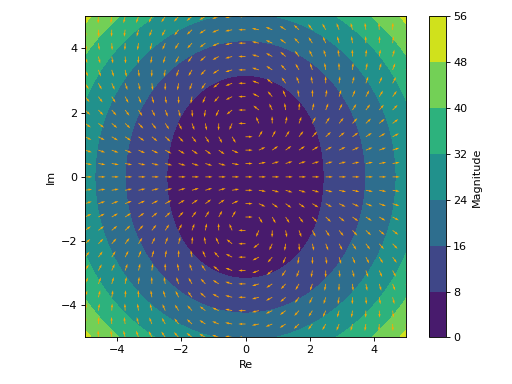
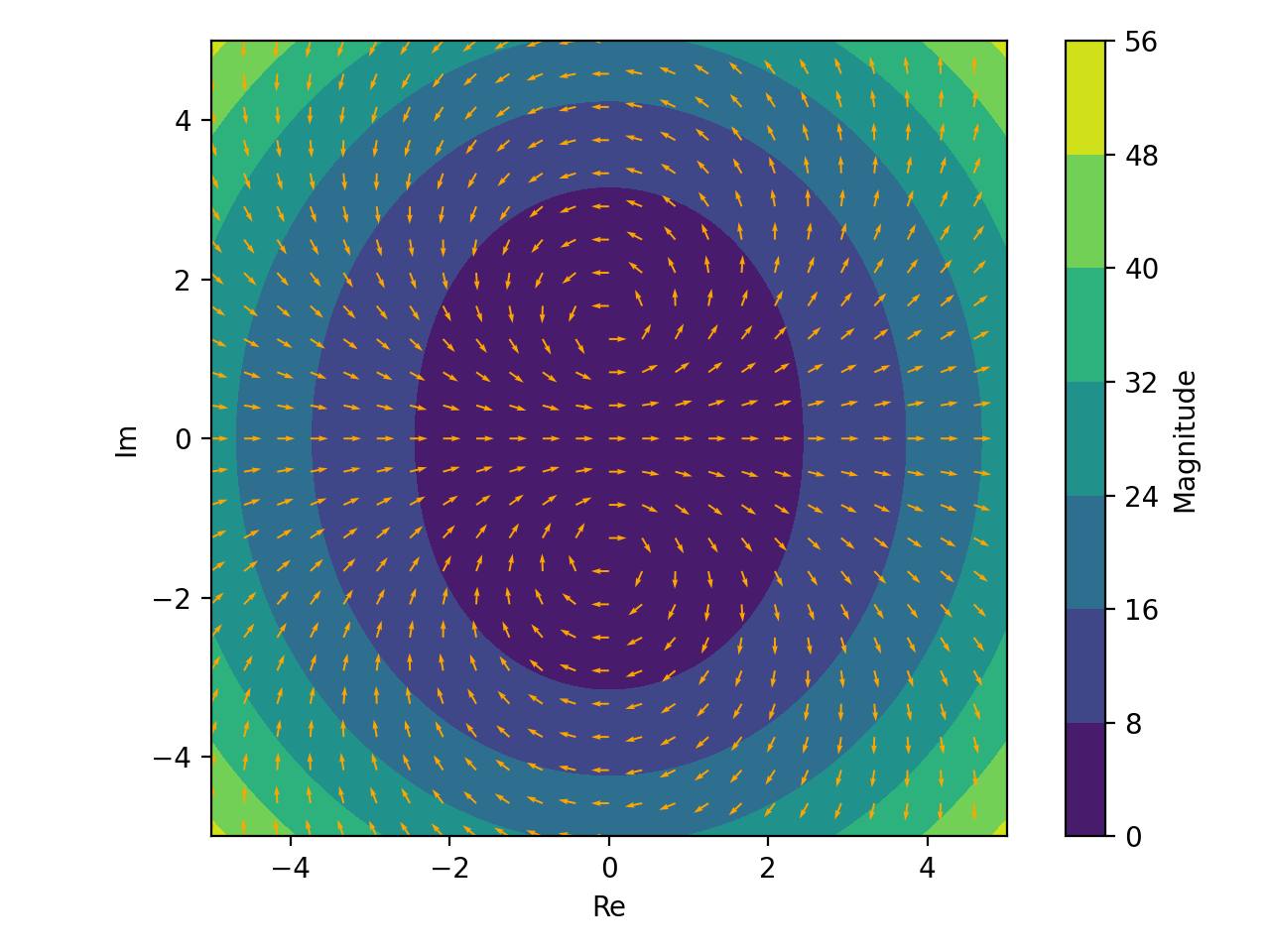
Quivers plot with normalize lengths and a contour plot in background representing the vector’s magnitude (a scalar field).
>>> expr = z**2 + 2
>>> plot_complex_vector(expr, (z, -5 - 5j, 5 + 5j),
...     quiver_kw=dict(color="orange"), normalize=True, grid=False)
Plot object containing:
[0]: contour: sqrt(4*(re(_x) - im(_y))**2*(re(_y) + im(_x))**2 + ((re(_x) - im(_y))**2 - (re(_y) + im(_x))**2 + 2)**2) for _x over (-5.0, 5.0) and _y over (-5.0, 5.0)
[1]: 2D vector series: [(re(_x) - im(_y))**2 - (re(_y) + im(_x))**2 + 2, 2*(re(_x) - im(_y))*(re(_y) + im(_x))] over (_x, -5.0, 5.0), (_y, -5.0, 5.0)
(
Source code,png,hires.png,pdf)
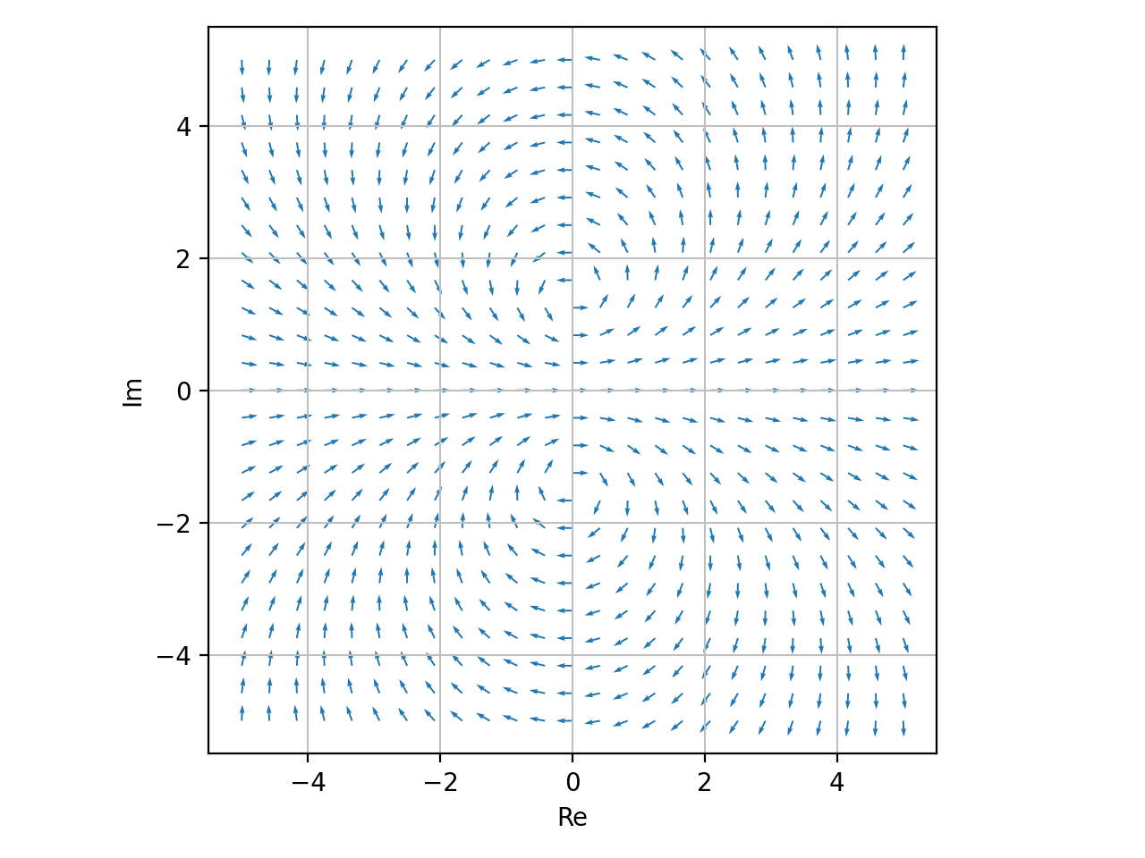
Only quiver plot with normalized lengths and solid color.
>>> plot_complex_vector(expr, (z, -5 - 5j, 5 + 5j),
...     scalar=False, use_cm=False, normalize=True)
Plot object containing:
[0]: 2D vector series: [(re(_x) - im(_y))**2 - (re(_y) + im(_x))**2 + 2, 2*(re(_x) - im(_y))*(re(_y) + im(_x))] over (_x, -5.0, 5.0), (_y, -5.0, 5.0)
(
Source code,png,hires.png,pdf)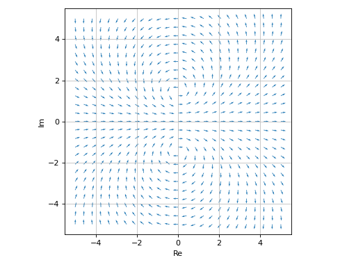
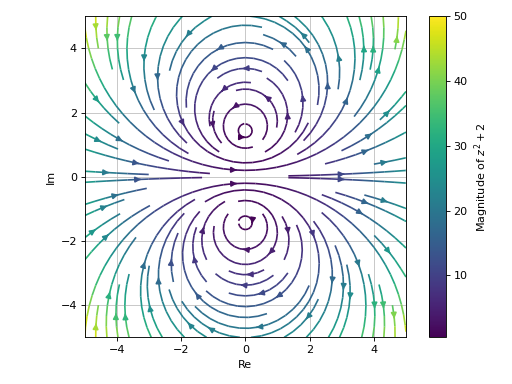
Only streamlines plot.
>>> plot_complex_vector(expr, (z, -5 - 5j, 5 + 5j),
...     "Magnitude of $%s$" % latex(expr),
...     scalar=False, streamlines=True)
Plot object containing:
[0]: 2D vector series: [(re(_x) - im(_y))**2 - (re(_y) + im(_x))**2 + 2, 2*(re(_x) - im(_y))*(re(_y) + im(_x))] over (_x, -5.0, 5.0), (_y, -5.0, 5.0)
(
Source code,png,hires.png,pdf)
Overlay the quiver plot to a domain coloring plot. By setting
n=26(even number) in the complex vector plot, the quivers won’t to cross the branch cut.>>> expr = z * log(2 * z) + 3 >>> p1 = plot_complex(expr, (z, -2-2j, 2+2j), grid=False, show=False) >>> p2 = plot_complex_vector(expr, (z, -2-2j, 2+2j), ... n=26, grid=False, scalar=False, use_cm=False, normalize=True, ... quiver_kw={"color": "k", "pivot": "tip"}, show=False) >>> (p1 + p2).show() >>> (p1 + p2) Plot object containing: [0]: complex domain coloring: z*log(2*z) + 3 for re(z) over (-2.0, 2.0) and im(z) over (-2.0, 2.0) [1]: 2D vector series: [(re(_x) - im(_y))*log(Abs(2*_x + 2*_y*I)) - (re(_y) + im(_x))*arg(_x + _y*I) + 3, (re(_x) - im(_y))*arg(_x + _y*I) + (re(_y) + im(_x))*log(Abs(2*_x + 2*_y*I))] over (_x, -2.0, 2.0), (_y, -2.0, 2.0)
(
Source code,png,hires.png,pdf)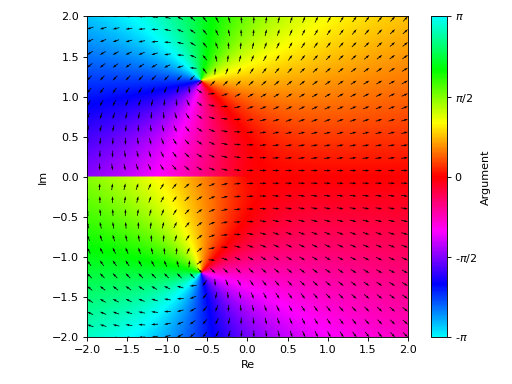
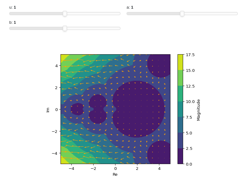
Interactive-widget plot. Refer to the interactive sub-module documentation to learn more about the
paramsdictionary. This plot illustrates:the use of
prange(parametric plotting range).the use of the
paramsdictionary to specify sliders in their basic form: (default, min, max).
from sympy import *
from spb import *
z, u, a, b = symbols("z u a b")
plot_complex_vector(
    log(gamma(u * z)), prange(z, -5*a - b*5j, 5*a + b*5j),
    params={
        u: (1, 0, 2),
        a: (1, 0, 2),
        b: (1, 0, 2)
    }, n=20, grid=False, use_latex=False,
    quiver_kw=dict(color="orange", headwidth=4))