0 - Evaluation algorithm

How does the plotting module works? Conceptually, it is very simple:

1. With lambdify it converts the symbolic expression to a function, which will be used for numerical evaluation.

2. It will evaluate the function over the specified domain. Usually, the default evaluation modules are Numpy and Scipy.

3. The numerical data can be post-processed and later plotted.

When it comes to 2D line plots we can either use:

• a meshing algorithm, which divides the specified range into n points (according to some strategy, for example linear or logarithm) over which the function will be evaluated. Usually, this approach is faster than the adaptive algorithm. This is the default algorithm used by the plotting module.

• an adaptive algorithm which is going to chose where to evaluate a function in order to obtain a smooth plot. The iterative procedure minimizes some loss function (loss_fn) and will stop when the adaptive_goal has been reached.

The numerical evaluation is subjected to the limitations of a particular module as well as that of the chosen evaluation strategy (adaptive vs meshing algorithm).

In this tutorial we are going to explore a few particular cases, understanding what’s going on and attempt to use different strategies in order to obtain a plot.

In particular, a few examples are dedicated to the limitations of the adaptive algorithm. We will understand when it is not appropriate to use it. Generally, if a function exhibits mid-to-high frequencies in relation to the plotting range, then it is better to switch to the uniform meshing algorithm.

We can also play with detect_poles and eps in order to detect singularities. The singularity-dection algorithm is extremely simple, as it doesn’t analyze the symbolic expression in any way: it only relies on the gradient of the numerical data, thus it is a post-processing step. This means than the user must know in advance if a function contains one or more singularities, eventually activating the detection algorithm and playing with the parameters in order to get the expected result. This is a try-and-repeat process until the user is satisfied with the result.

>>> from sympy import *
>>> from spb import *
>>> x = symbols("x")

(Source code)

Example - Dealing with ‘Not A Number’

The adaptve algorithm requires the expression to be defined at least in a subset of the specified plotting range. For example:

>>> plot(log(x), (x, -5, 5), adaptive=True)
Plot object containing:
[0]: cartesian line: log(x) for x over (-5.0, 5.0)

(Source code, png)

It is well known that log(x) is defined for x > 0. The adaptive algorithm evaluated the function over the entire range x in [-5, 5]: obviously, for x <= 0 it returned nan (not a number), whereas for x > 0 it returned a real finite number. The adaptive evaluation succeeded because it computed at least one finite number, with which the algorithm was able to minimize the loss function loss_fn and reached the required adaptive_goal.

What happens if we try to evaluate a function over a range in which it is not defined? For example, plot(log(x), (x, -5, 0), adaptive=True). Here, the evaluation will never be able to stop because it is impossible to minimize the loss function with the computed nan values. The algorithm keeps running forever, sampling more and more points.

Differently, the meshing algorithm evaluates the function over a finite number of points, hence it will create an empty plot, because log(x) is not defined for x <= 0.

>>> plot(log(x), (x, -5, 0), adaptive=False)
Plot object containing:
[0]: cartesian line: log(x) for x over (-5.0, 0.0)

(Source code, png)

Example - Evaluation modules

Plotting an expression that evaluates to huge numbers is no easy task either. For example:

>>> expr = (factorial(365) / factorial(365 - x)) / 365**x
>>> # plot(expr, (x, 0, 100), adaptive=True)

(Source code)

If we execute that plot command, the computation will never finish. Let’s debug what’s going on by creating a numerical function with lambdify:

>>> f = lambdify(x, expr)
>>> import inspect
>>> print(inspect.getsource(f))    

(Source code)

def _lambdifygenerated(x):
    return 25104128675558732292929443748812027705165520269876079766872595193901106138220937419666018009000254169376172314360982328660708071123369979853445367910653872383599704355532740937678091491429440864316046925074510134847025546014098005907965541041195496105311886173373435145517193282760847755882291690213539123479186274701519396808504940722607033001246328398800550487427999876690416973437861078185344667966871511049653888130136836199010529180056125844549488648617682915826347564148990984138067809999604687488146734837340699359838791124995957584538873616661533093253551256845056046388738129702951381151861413688922986510005440943943014699244112555755279140760492764253740250410391056421979003289600000000000000000000000000000000000000000000000000000000000000000000000000000000000000000*365**(-x)/factorial(365 - x)

We can see a very large integer number. Now, let’s try to evaluate the function: for example f(5). We will get: OverflowError: int too large to convert to float. We could change the evaluation module on the lambdified function, but the result wouldn’t change: Python is trying to convert an integer number to a Python’s float, which is too small to hold that number.

Going back to the plot command, nan will be returned whenever an OverflowError is raised. Hence, this is a similar situation to the previous example: the adaptive algorithm can’t mizimize the loss function, as such it runs forever.

Now, let’s try to switch to the meshing algorithm:

>>> p = plot(expr, (x, 0, 100), adaptive=False)

(Source code, png)

Again, the plot is empty because an OverflowError was raised (thus nan was returned) for every evaluation point.

We can try to change the expression by preventing the evaluation of the factorial:

>>> expr = (factorial(365, evaluate=False) / factorial(365 - x)) / 365**x
>>> f = lambdify(x, expr)
>>> f(5)
nan

(Source code)

Again, we are getting a nan. We could try to change the evaluation module to math, but then it would raise: OverflowError: int too large to convert to float. Alternatively, we can try mpmath:

>>> f = lambdify(x, expr, modules="mpmath")
>>> f(5)
mpf('0.97286442630020653')

(Source code)

Why is it working? Differently from Python and Numpy, whose float has a fixed size, mpmath uses arbitrary-precision floating-point arithmetic. So, we can try to plot the expression with mpmath, taking into consideration that the function will be slower to evaluate:

>>> p = plot(expr, (x, 0, 100), adaptive=True, modules="mpmath")

(Source code, png)

Then, the plot command will also work when switching to a meshing algorithm (adaptive=False).

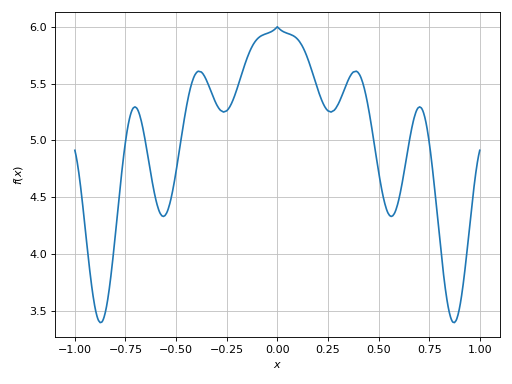
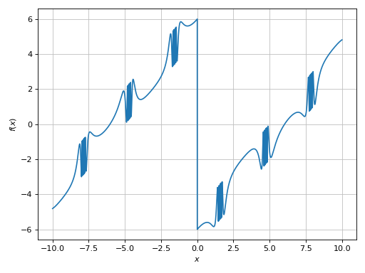
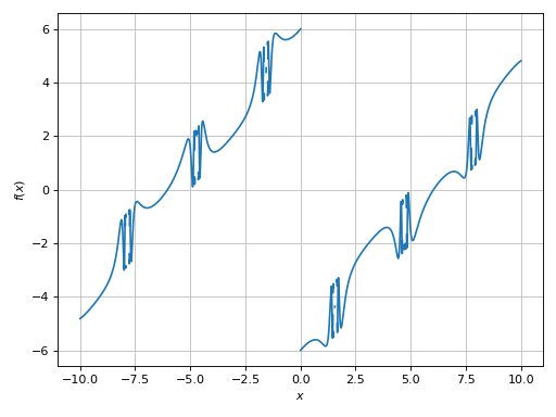
Example - Smoothness

>>> expr = x * sin(20 * x) - Abs(2 * x) + 6
>>> plot(expr, (x, -1, 1), adaptive=True)
Plot object containing:
[0]: cartesian line: x*sin(20*x) - 2*Abs(x) + 6 for x over (-1.0, 1.0)

(Source code, png)

Here the plotting module used the adaptive algorithm. In the provided range, the function has a relatively low frequency, so the adaptive algorithm (using the default options) was able to create a smooth plot.

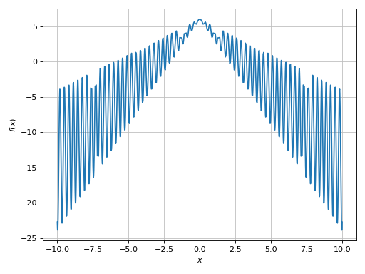
Let’s try to use a wider plot range:

>>> plot(expr, (x, -10, 10), adaptive=True)
Plot object containing:
[0]: cartesian line: x*sin(20*x) - 2*Abs(x) + 6 for x over (-10.0, 10.0)

(Source code, png)

This is a case of mid-to-high frequencies (in relation to the plotting range used). We can see a few “missed” spikes. If we zoom into the plot, we will also see a very poor smoothness. The adaptive algorithm worked as expected: it minimized some loss function (loss_fn) until the default goal was reached (adaptive_goal=0.01). To improve the output we can either:

1. decrease the value of adaptive_goal: depending on the value, the execution will slow down quite a bit.

2. switch to the uniform meshing algorithm and increase the number of discretization points. This techniques will use Numpy arrays for the evaluation, so we are going to get relatively good performances.

Let’s try to decrease adaptive_goal by one order of magnitude:

>>> plot(expr, (x, -10, 10), adaptive=True, adaptive_goal=1e-03)
Plot object containing:
[0]: cartesian line: x*sin(20*x) - 2*Abs(x) + 6 for x over (-10.0, 10.0)

(Source code, png)

The resulting plot is much better: by zooming into it we will see a nice smooth line. However, the evaluation was significantly slower!

For comparison, let’s try to use the uniform meshing algorithm. This will create a nice smooth plot almost instantly:

>>> plot(expr, (x, -10, 10), adaptive=False, n=1e04)
Plot object containing:
[0]: cartesian line: x*sin(20*x) - 2*Abs(x) + 6 for x over (-10.0, 10.0)

(Source code, png)

Example - Discontinuities 1

Let’s execute the following code:

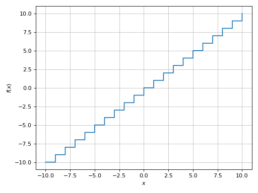
>>> plot(floor(x), adaptive=True)
Plot object containing:
[0]: cartesian line: floor(x) for x over (-10.0, 10.0)

(Source code, png)

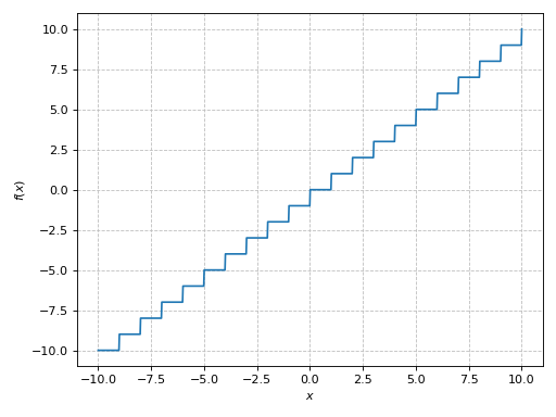
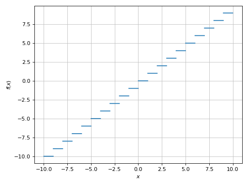
Because we are dealing with a floor function, there are discontinuities between the horizontal segments. Let’s activate the singularity-detection algorithm:

>>> plot(floor(x), adaptive=True, detect_poles=True)
Plot object containing:
[0]: cartesian line: floor(x) for x over (-10.0, 10.0)

(Source code, png)

We can also use the uniform meshing strategy, but we would have to use a sufficiently high number of discretization points:

>>> plot(floor(x), adaptive=False, n=1e04, detect_poles=True)
Plot object containing:
[0]: cartesian line: floor(x) for x over (-10.0, 10.0)

(Source code, png)

Alternatively, we can provide a list of exclusion points:

>>> plot(floor(x), (x, -9.5, 9.5), exclude=list(range(-10, 11)))
Plot object containing:
[0]: cartesian line: floor(x) for x over (-9.5, 9.5)

(Source code, png)

Example - Discontinuities 2

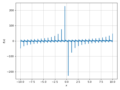
Let’s try another example of a function containing the floor function. This is a case of mid-to-high frequencies in relation to the plotting range, so it is advisable to set adaptive=False:

>>> expr = tan(floor(30 * x)) + x / 8
>>> plot(expr, adaptive=False, n=1e04)
Plot object containing:
[0]: cartesian line: x/8 + tan(floor(30*x)) for x over (-10.0, 10.0)

(Source code, png)

There is a wide spread along the y-direction. Let’s limit it:

>>> plot(expr, adaptive=False, n=1e04, ylim=(-10, 10))
Plot object containing:
[0]: cartesian line: x/8 + tan(floor(30*x)) for x over (-10.0, 10.0)

(Source code, png)

Let’s remember that we are dealing with a floor function, so ther should be distinct segments in the plot:

>>> plot(expr, adaptive=False, n=1e04, ylim=(-10, 10), detect_poles=True)
Plot object containing:
[0]: cartesian line: x/8 + tan(floor(30*x)) for x over (-10.0, 10.0)

(Source code, png)

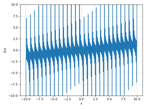
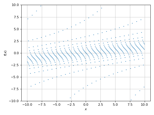
Example - Discontinuities 3

Using the adaptive algorith, the following example will probably take forever to plot:

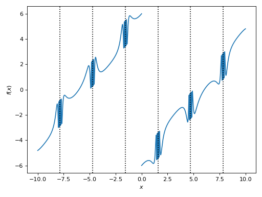
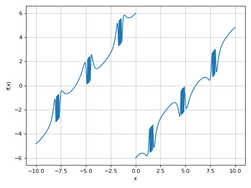
>>> expr = sign(x) * (sin(1 - 1 / cos(x)) + Abs(x) - 6)
>>> # plot(expr, adaptive=True)

(Source code)

We can stop the execution.

Why is it so slow? Let’s look at the argument of the sin function (the frequency): as cos(x) approaches 0, the frequency goes to infinity. The adaptive algorithm is trying to resolve this situation, but it’s going to take a very long time. We have two options:

1. increase the value of adaptive_goal, thus reducing the smoothness of the function and potentially loosing important information.

2. use the uniform meshing algorithm.

Let’s try the second approach:

>>> plot(expr, adaptive=False, n=1e04)
Plot object containing:
[0]: cartesian line: (sin(1 - 1/cos(x)) + Abs(x) - 6)*sign(x) for x over (-10.0, 10.0)

(Source code, png)

Much better, but the plot is still misleading: there is a sign function in the expression, so there must be some discontinuities. Let’s activate the singularity detection algorithm:

>>> plot(expr, adaptive=False, n=1e04, detect_poles=True)
Plot object containing:
[0]: cartesian line: (sin(1 - 1/cos(x)) + Abs(x) - 6)*sign(x) for x over (-10.0, 10.0)

(Source code, png)

It worked, but it did too much: it has also disconnected the high frequency regions. We can try to get a better visualization by:

• increasing the number of discretization points.

• reducing the eps parameter. The smaller this parameter, the higher the threshold used by the singularity detection algorithm.

This is going to take a few attempts:

>>> plot(expr, adaptive=False, n=5e04, detect_poles=True, eps=1e-04)
Plot object containing:
[0]: cartesian line: (sin(1 - 1/cos(x)) + Abs(x) - 6)*sign(x) for x over (-10.0, 10.0)

(Source code, png)

Finally, we can enable the symbolic poles detection algorith to visualize where this function is not defined:

>>> plot(expr, adaptive=False, n=5e04, detect_poles="symbolic", eps=1e-04, grid=False)
Plot object containing:
[0]: cartesian line: (sin(1 - 1/cos(x)) + Abs(x) - 6)*sign(x) for x over (-10.0, 10.0)

(Source code, png)

Example - Discontinuities 4

>>> expr = sin(20 * x) + sign(sin(19.5 * x)) + x
>>> plot(expr, adaptive=True)
Plot object containing:
[0]: cartesian line: x + sin(20*x) + sign(sin(19.5*x)) for x over (-10.0, 10.0)

(Source code, png)

The expression contains a sign function, so there should be discontinuities. Also, if we zoom into the plot we see that it is not very “smooth”: the frequency is quite high with respect to the plotting range. So:

>>> plot(expr, adaptive=False, n=1e04, detect_poles=True)
Plot object containing:
[0]: cartesian line: x + sin(20*x) + sign(sin(19.5*x)) for x over (-10.0, 10.0)

(Source code, png)

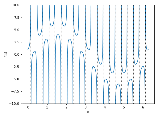
Example - Discontinuities 5

Another function having many singularities:

>>> expr = 1 / cos(10 * x) + 5 * sin(x)
>>> plot(expr, adaptive=True)
Plot object containing:
[0]: cartesian line: 5*sin(x) + 1/cos(10*x) for x over (-10.0, 10.0)

(Source code, png)

Again, a very big spread along the y-direction. We need to limit it:

>>> plot(expr, adaptive=True, ylim=(-10, 10))
Plot object containing:
[0]: cartesian line: 5*sin(x) + 1/cos(10*x) for x over (-10.0, 10.0)

(Source code, png)

The plot is clearly misleading. We can guess that it has a mid-to-high frequency with respect to the plotting range. Also, by looking at the expression there must be singularities:

>>> plot(expr, ylim=(-10, 10), adaptive=False, n=1e04, detect_poles=True)
Plot object containing:
[0]: cartesian line: 5*sin(x) + 1/cos(10*x) for x over (-10.0, 10.0)

(Source code, png)

We can improve it even further by reducing the eps parameter:

>>> plot(expr, ylim=(-10, 10), adaptive=False, n=1e04, detect_poles=True, eps=1e-04)
Plot object containing:
[0]: cartesian line: 5*sin(x) + 1/cos(10*x) for x over (-10.0, 10.0)

(Source code, png)

Alternatively, we can provide a list of exclusion points. The following example executes solveset(cos(10 * x)), which returns a set solution. This set is given to the exclude keyword argument, which will attempt to extract suitable numerical solutions for the exclusion points:

>>> expr = 1 / cos(10 * x) + 5 * sin(x)
>>> plot(expr, ylim=(-10, 10), exclude=solveset(cos(10 * x)))
Plot object containing:
[0]: cartesian line: 5*sin(x) + 1/cos(10*x) for x over (-10.0, 10.0)

(Source code, png)

Example - Discontinuities 6

Let’s try to plot the Gamma function:

>>> expr = gamma(x)
>>> plot(expr, (x, -5, 5), adaptive=True)
Plot object containing:
[0]: cartesian line: gamma(x) for x over (-5.0, 5.0)

(Source code, png)

A very big spread along the y-direction. We need to limit it:

>>> plot(expr, (x, -5, 5), ylim=(-5, 5), adaptive=True)
Plot object containing:
[0]: cartesian line: gamma(x) for x over (-5.0, 5.0)

(Source code, png)

Here we can see a few discontinuities. Let’s enable the singularity detection algorithm:

>>> plot(expr, (x, -5, 5), ylim=(-5, 5), adaptive=False, n=2e04, detect_poles=True, eps=1e-04)
Plot object containing:
[0]: cartesian line: gamma(x) for x over (-5.0, 5.0)

(Source code, png)