5 - Colors and Colormaps

Backends apply default rendering settings to the objects of the figure depending on the type of plot we are generating. For example, when executing the plot() function, backends use solid color and solid line style. When executing plot_parametric() or plot3d(), they use colormaps.

In this tutorial we are going to see how to modify this rendering options. It is assumed that the default backend is Matplotlib, both for 2D and 3D plots.

Change rendering options

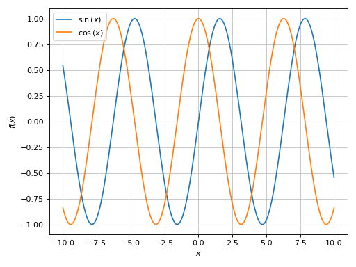
Let’s start by plotting a couple of expressions. By default, the backend will apply a colorloop so that each expression gets a unique color.

from sympy import *
from spb import *
var("x, y")
plot(sin(x), cos(x))

(Source code, png)

We can modify the styling of the lines by providing backend-specific commands through the rendering_kw argument (or keyword argument), which will be passed directly to the backend-specific function responsible to draw lines.

Some plot functions might create multiple data series about the same symbolic expression, so it exposes different rendering-related keyword arguments. For example, plot_vector combines a contour plot with a quiver (or streamline) plot, hence it exposes contour_kw, quiver_kw and stream_kw.

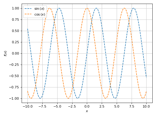
Let’s try to apply a dashed line style:

# provide the rendering_kw argument
plot(sin(x), cos(x), dict(linestyle="--"))
# alternatively, we can set the rendering_kw keyword argument
# plot(sin(x), cos(x), rendering_kw=dict(linestyle="--"))

(Source code, png)

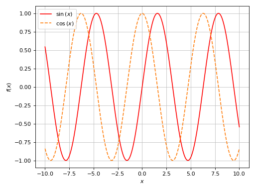
As we can see, the same style has been applied to every series. What if we would like to apply different styles to different series? We can create a tuple of the form (expr, label [optional], rendering_kw [optional]) for each expression, or we can provide a list of dictionaries to the rendering_kw keyword argument, where the number of dictionaries must be equal to the number of expressions being plotted. For example:

plot((sin(x), dict(color="red")), (cos(x), dict(linestyle="--")))
# alternatively, set rendering_kw to a list of dictionaries
# plot(sin(x), cos(x), rendering_kw=[dict(color="red"), dict(linestyle="--")])

(Source code, png)

Alternatively, we can create different plots and combine them together:

p1 = plot(sin(x), dict(color="red"), show=False)
p2 = plot(cos(x), dict(linestyle="--"), show=False)
p3 = p1 + p2
p3.show()

(Source code, png)

Note that the second series, cos(x), is using the automatic color provided by the backend.

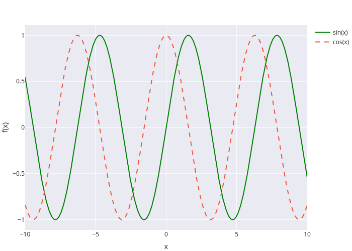
Now, let’s try to do the same with Plotly. Note that the rendering options are different!

from sympy import *
from spb import *
var("x, y")
plot((sin(x), dict(line_color="green")), (cos(x), dict(line_dash="dash")), backend=PB)

(Source code, png)

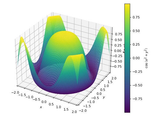
Let’s now use same concepts with a 3D plot. This is the default look:

plot3d(cos(x**2 + y**2), (x, -2, 2), (y, -2, 2), use_cm=True)

(Source code, png)

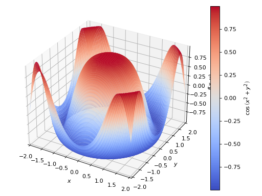
Now, let’s change the colormap:

import matplotlib.cm as cm
plot3d(cos(x**2 + y**2), (x, -2, 2), (y, -2, 2), dict(cmap=cm.coolwarm), use_cm=True)

(Source code, png)

Custom color loop and colormaps

We can also modify the color loop and the colormaps used by the backend. Each backend exposes the colorloop and colormaps class attributes, which are empty lists:

print(MB.colorloop)
print(MB.colormaps)

[]
[]

We can fill these lists with our preferred colors or colormaps. For example:

import matplotlib.cm as cm
MB.colorloop = cm.Dark2.colors
plot(sin(x), cos(x), sin(x) * cos(x))

(Source code, png)

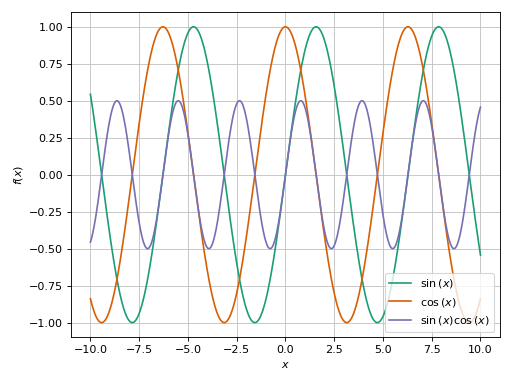
Note that cm.Dark2.colors returns a list of colors. By comparing this picture with the ones at the beginning, we can confirm that the colorloop has changed.

After setting these two class attribute, every plot will use the new colors, until the kernel is restarted or the attributes are set to empty lists.

Let’s try a 3D plot with default colormaps:

from sympy import *
from spb import *
var("x, y")
expr = cos(x**2 + y**2)
plot3d(
    (expr, (x, -2, 0), (y, -2, 0)),
    (expr, (x, 0, 2), (y, -2, 0)),
    (expr, (x, -2, 0), (y, 0, 2)),
    (expr, (x, 0, 2), (y, 0, 2)),
    n = 20, backend=PB, use_cm=True
)

(Source code, png)

Now, let’s change the colormaps:

from sympy import *
from spb import *
import colorcet as cc
import matplotlib.cm as cm
var("x, y")
expr = cos(x**2 + y**2)
PB.colormaps = ["solar", "aggrnyl", cm.coolwarm, cc.kbc]
plot3d(
    (expr, (x, -2, 0), (y, -2, 0)),
    (expr, (x, 0, 2), (y, -2, 0)),
    (expr, (x, -2, 0), (y, 0, 2)),
    (expr, (x, 0, 2), (y, 0, 2)),
    n = 20, backend=PB, use_cm=True
)

(Source code, png)

Note that all backend are able to use colormaps from a different plotting library!