K3DBackend
- class spb.backends.k3d.K3DBackend(*args, **kwargs)[source]
A backend for plotting SymPy’s symbolic expressions using K3D-Jupyter.
- Parameters:
- aspectstr, tuple, list, dict
Set the aspect ratio.
Possible values for Matplotlib (only works for a 2D plot):
"auto": Matplotlib will fit the plot in the vibile area."equal": sets equal spacing.tuple containing 2 float numbers, from which the aspect ratio is computed. This only works for 2D plots.
Possible values for Plotly:
"equal": sets equal spacing on the axis of a 2D plot.For 3D plots:
"cube": fix the ratio to be a cube"data": draw axes in proportion of their ranges"auto": automatically produce something that is well proportioned using ‘data’ as the default.manually set the aspect ratio by providing a dictionary. For example:
dict(x=1, y=1, z=2)forces the z-axis to appear twice as big as the other two.
Possible values for Bokeh:
"equal": sets equal spacing.
- ax
An existing Matplotlib’s Axes over which the symbolic expressions will be plotted.
- axisbool
Show the axis in the figure. Default value: True.
- axis_centerstr, tuple
Set the location of the intersection between the horizontal and vertical axis in a 2D plot. It only works with Matplotlib and it can receive the following values:
None: traditional layout, with the horizontal axis fixed on the bottom and the vertical axis fixed on the left. This is the default value.a tuple
(x, y)specifying the exact intersection point.'center': center of the current plot area.'auto': the intersection point is automatically computed.
- camera
Set the camera position for 3D plots.
For Matplotlib, it can be a dictionary of keyword arguments that will be passed to the
Axes3D.view_initmethod. Refer to the following link for more information: https://matplotlib.org/stable/api/_as_gen/mpl_toolkits.mplot3d.axes3d.Axes3D.html#mpl_toolkits.mplot3d.axes3d.Axes3D.view_initFor Plotly, it can be a dictionary of keyword arguments that will be passed to the layout’s
scene_camera. Refer to the following link for more information: https://plotly.com/python/3d-camera-controls/For K3D-Jupyter, it is list of 9 numbers, namely:
x_cam, y_cam, z_cam: the position of the camera in the scenex_tar, y_tar, z_tar: the position of the target of the camerax_up, y_up, z_up: components of the up vector
- colorlooplist, tuple
List of colors to be used in line plots or solid color surfaces.
- colormapslist, tuple
List of color maps to render surfaces.
- cyclic_colormapslist, tuple
List of cyclic color maps to render complex series (the phase/argument ranges over [-pi, pi]).
- fig
Get or set the figure where to plot into.
- gridbool, dict
Toggle the visibility of major grid lines. A dictionary of keyword arguments can be passed to customized the appearance of the grid lines:
- hookslist
List of functions expecting one argument, the current plot object, which allows users to further customize the appearance of the plot before it is shown on the screen. The hooks are executed:
after the figure has been initialized and populated with numerical data.
after the existing renderers update the visualization because the user interacted with some widget.
Note: let
pbe the plot object. Then, the user can access the figure withp.fig. In case ofspb.backends.matplotlib.MatplotlibBackend, the user can also retrieve the axes in which data was added withp.ax.- invert_x_axisbool
Allow to invert x-axis if the range is given as (symbol, max, min) instead of (symbol, min, max). Default value: False.
- legendbool
Toggle the visibility of the legend. If None, the backend will automatically determine if it is appropriate to show it. Default value: None.
- minor_gridbool, dict
Toggle the visibility of minor grid lines. A dictionary of keyword arguments can be passed to customized the appearance of the grid lines:
- polar_axisbool
If True, the backend will attempt to use polar axis, otherwise it uses cartesian axis. This is only supported for 2D plots. Default value: False.
- show_labelbool
Show/hide labels of the expressions on the K3D-Jupyter’s user interface. Default value: False.
- size
Set the size of the plot, (width, height). For Matplotlib, the size is measured in inches. For Bokeh, Plotly and K3D-Jupyter, the size is in pixel.
- themestr
Theme to be used to style the figure. Depending on the backend being used, several themes may be available.
- title
Title of the plot. It can be:
a string.
a callable receiving a single argument, use_latex, which must return a string.
a tuple of the form (format_str, symbol 1, symbol 2, etc.), which creates an output string when parameters symbol 1, symbol 2, etc. receive numerical values from the widgets. This operation mode only works when creating interactive data series (ie, specifying the
paramsdictionary).
- update_eventbool
If True and the backend supports such functionality, events like drag and zoom will trigger a recompute of the data series within the new axis limits. Default value: False.
- use_latexbool
Turn on/off the rendering of latex labels. If the backend doesn’t support latex, it will render the string representations instead. Default value: True.
- x_ticks_formattertick_formatter_multiples_of
An object of type
tick_formatter_multiples_ofwhich will be used to place tick values at each multiple of a specified quantity, along the x-axis.- xlabel
Label of the x-axis. It can be:
a string.
a callable receiving a single argument, use_latex, which must return a string.
a tuple of the form (format_str, symbol 1, symbol 2, etc.), which creates an output string when parameters symbol 1, symbol 2, etc. receive numerical values from the widgets. This operation mode only works when creating interactive data series (ie, specifying the
paramsdictionary).
- xlim
Limit the figure’s x-axis to the specified range. The tuple must be in the form (min_val, max_val).
- xscaleNoneType, str
If the backend supports it, the x-direction will use the specified scale. Note that none of the backends support logarithmic scale for 3D plots. Possible options: [‘linear’, ‘log’, None] Default value: ‘linear’.
- y_ticks_formattertick_formatter_multiples_of
An object of type
tick_formatter_multiples_ofwhich will be used to place tick values at each multiple of a specified quantity, along the y-axis.- ylabel
Label of the y-axis. It can be:
a string.
a callable receiving a single argument, use_latex, which must return a string.
a tuple of the form (format_str, symbol 1, symbol 2, etc.), which creates an output string when parameters symbol 1, symbol 2, etc. receive numerical values from the widgets. This operation mode only works when creating interactive data series (ie, specifying the
paramsdictionary).
- ylim
Limit the figure’s y-axis to the specified range. The tuple must be in the form (min_val, max_val).
- yscaleNoneType, str
If the backend supports it, the y-direction will use the specified scale. Note that none of the backends support logarithmic scale for 3D plots. Possible options: [‘linear’, ‘log’, None] Default value: ‘linear’.
- zlabel
Label of the z-axis. It can be:
a string.
a callable receiving a single argument, use_latex, which must return a string.
a tuple of the form (format_str, symbol 1, symbol 2, etc.), which creates an output string when parameters symbol 1, symbol 2, etc. receive numerical values from the widgets. This operation mode only works when creating interactive data series (ie, specifying the
paramsdictionary).
- zlim
Limit the figure’s z-axis to the specified range. The tuple must be in the form (min_val, max_val).
- zscaleNoneType, str
If the backend supports it, the z-direction will use the specified scale. Note that none of the backends support logarithmic scale for 3D plots. Possible options: [‘linear’, ‘log’, None] Default value: ‘linear’.
Methods
append(series)
Adds another series to this plot.
draw()
Loop over data renderers, generates numerical data and add it to the figure. Note that this method doesn’t show the plot.
extend(plot_or_series)
Adds all series from another plot to this plot.
save(path, **kwargs)
Export the plot to a static picture or to an interactive html file.
show()
Visualize the plot on the screen.
update_interactive(params)
Implement the logic to update the data generated by interactive-widget plots.
See also
Plot,MatplotlibBackend,PlotlyBackend,BokehBackend,plot3d
Notes
After the installation of this plotting module, try one of the examples of
plot3dwith this backend. If no figure is visible in the output cell, follow this procedure:Save the Notebook.
Close Jupyter server.
Run the following commands, which are going to install the Jupyter extension for K3D:
jupyter nbextension install –user –py k3d
jupyter nbextension enable –user –py k3d
Restart jupyter notebook
Open the previous notebook and execute the plot command.
- K3DBackend.fig
Returns the figure.
- spb.backends.k3d.K3DBackend.append(self, series)
Adds another series to this plot.
- Parameters:
- argBaseSeries
An instance of BaseSeries which will be used to generate the numerical data.
See also
Examples
Consider two Plot objects, p1 and p2. To add the second plot’s first series object to the first, use the append method, like so:
>>> from sympy import symbols
>>> from spb import plot
>>> x = symbols('x')
>>> p1 = plot(x*x, show=False)
>>> p2 = plot(x, show=False)
>>> p1.append(p2[0])
>>> p1
Plot object containing:
[0]: cartesian line: x**2 for x over (-10, 10)
[1]: cartesian line: x for x over (-10, 10)
>>> p1.show()
(
Source code,png)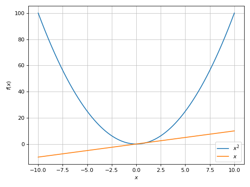
- spb.backends.k3d.K3DBackend.extend(self, plot_or_series)
Adds all series from another plot to this plot.
- Parameters:
- plot_or_series
Plot or sequence of BaseSeries
See also
Examples
Consider two Plot objects, p1 and p2. To add the second plot to the first, use the extend method, like so:
>>> from sympy import symbols
>>> from spb import plot
>>> x = symbols('x')
>>> p1 = plot(x**2, show=False)
>>> p2 = plot(x, -x, show=False)
>>> p1.extend(p2)
>>> p1
Plot object containing:
[0]: cartesian line: x**2 for x over (-10, 10)
[1]: cartesian line: x for x over (-10, 10)
[2]: cartesian line: -x for x over (-10, 10)
>>> p1.show()
(
Source code,png)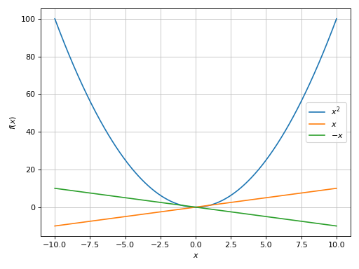
- spb.backends.k3d.K3DBackend.save(self, path, **kwargs)
Export the plot to a static picture or to an interactive html file.
Notes
K3D-Jupyter is only capable of exporting:
‘.png’ pictures: refer to [1] to visualize the available keyword arguments.
‘.html’ files: this requires the
msgpack[2] python module to be installed.When exporting a fully portable html file, by default the required Javascript libraries will be loaded with a CDN. Set
include_js=Trueto include all the javascript code in the html file: this will create a bigger file size, but can be run without internet connection.
References
- spb.backends.k3d.K3DBackend.show(self)
Visualize the plot on the screen.
- spb.backends.k3d.K3DBackend.update_interactive(self, params)
Implement the logic to update the data generated by interactive-widget plots.
- Parameters:
- paramsdict
Map parameter-symbols to numeric values.