Plot
About the Implementation
Why different backends inheriting from the Plot class? Why not using
something like holoviews, which allows to plot
numerical data with different plotting libraries using a common interface?
In short:
Holoviews only support Matplotlib, Bokeh, Plotly. This would make impossible to add support for further libraries, such as K3D, …
Not all needed features might be implemented on Holoviews. Think for example to plotting a gradient-colored line. Matplotlib and Bokeh are able to visualize it correctly, Plotly doesn’t support this functionality. By not using Holoviews, we can more easily implement some work around.
- class spb.backends.base_backend.Plot(*args, **kwargs)[source]
Base class for all backends. A backend represents the plotting library, which implements the necessary functionalities in order to use SymPy plotting functions.
How the plotting module works:
The user creates the symbolic expressions and calls one of the plotting functions.
The plotting functions generate a list of instances of
BaseSeries, containing the necessary information to generate the appropriate numerical data and create the proper visualization (eg the expression, ranges, series name, …).The plotting functions instantiate the
Plotclass, which stores the list of series and the main attributes of the plot (eg axis labels, title, etc.). Among the keyword arguments, there must bebackend=, where a subclass ofPlotcan be specified in order to use a particular plotting library.Each data series will be associated to a corresponding renderer, which receives the numerical data and add it to the figure. A renderer is also responsible to keep objects up-to-date when interactive-widgets plots are used. The figure is populated with numerical data when the
show()method or thefigattribute are called.
The backend should check if it supports the data series that it’s given. Please, explore
MatplotlibBackendsource code to understand how a backend should be coded.Also note that setting attributes to plot objects or to data series after they have been instantiated is strongly unrecommended, as it is not guaranteed that the figure will be updated.
- Parameters:
- titlestr, optional
Set the title of the plot. Default to an empty string.
- xlabel, ylabel, zlabelstr, optional
Set the labels of the plot. Default to an empty string.
- legendbool, optional
Show or hide the legend. By default, the backend will automatically set it to True if multiple data series are shown.
- xscale, yscale, zscalestr, optional
Discretization strategy for the provided domain along the specified direction. Can be either ‘linear’ or ‘log’. Default to ‘linear’. If the backend supports it, the specified direction will use the user-provided scale. By default, all backends uses linear scales for both axis. None of the backends support logarithmic scale for 3D plots.
- gridbool, optional
Show/Hide the grid. The default value depends on the backend.
- xlim, ylim, zlim(float, float), optional
Focus the plot to the specified range. The tuple must be in the form (min_val, max_val).
- aspect(float, float) or str, optional
Set the aspect ratio of the plot. It only works for 2D plots. The values depends on the backend. Read the interested backend’s documentation to find out the possible values.
- backendPlot
The subclass to be used to generate the plot.
- size(float, float) or None, optional
Set the size of the plot, (width, height). Default to None.
See also
MatplotlibBackend,PlotlyBackend,BokehBackend,K3DBackend
Notes
In order to be used by SymPy plotting functions, a backend must implement the following methods and attributes:
show(self): used to loop over the data series, generate the numerical data, plot it and set the axis labels, title, …save(self, path, **kwargs): used to save the current plot to the specified file path.self._fig: an instance attribute to store the backend-specific plot object, which can be retrieved with thePlot.figattribute. This object can then be used to further customize the resulting plot, using backend-specific commands.update_interactive(self, params): this method receives a dictionary mapping parameters to their values from theiplotfunction, which are going to be used to update the objects of the figure.
Examples
Combine multiple plots together to create a new plot:
>>> from sympy import symbols, sin, cos, log, S
>>> from spb import plot, plot3d
>>> x, y = symbols("x, y")
>>> p1 = plot(sin(x), cos(x), show=False)
>>> p2 = plot(sin(x) * cos(x), log(x), show=False)
>>> p3 = p1 + p2
>>> p3.show()
(
Source code,png)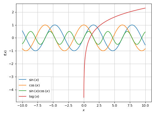
Use the index notation to access the data series. Let’s generate the numerical data associated to the first series:
>>> p1 = plot(sin(x), cos(x), show=False)
>>> xx, yy = p1[0].get_data()
Create a new backend with a custom colorloop:
>>> from spb.backends.matplotlib import MB
>>> class MBchild(MB):
...     colorloop = ["r", "g", "b"]
>>> plot(sin(x) / 3, sin(x) * S(2) / 3, sin(x), backend=MBchild)
Plot object containing:
[0]: cartesian line: sin(x)/3 for x over (-10.0, 10.0)
[1]: cartesian line: 2*sin(x)/3 for x over (-10.0, 10.0)
[2]: cartesian line: sin(x) for x over (-10.0, 10.0)
(
Source code,png)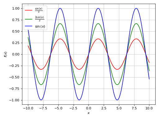
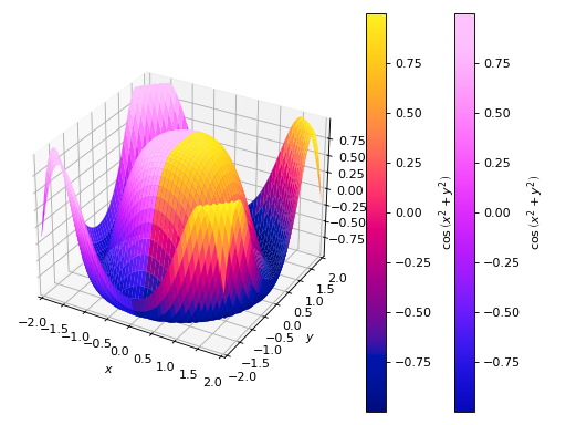
Create a new backend with custom color maps for 3D plots. Note that it’s possible to use Plotly/Colorcet/Matplotlib colormaps interchangeably.
>>> from spb.backends.matplotlib import MB
>>> import colorcet as cc
>>> class MBchild(MB):
...     colormaps = ["plotly3", cc.bmy]
>>> plot3d(
...     (cos(x**2 + y**2), (x, -2, 0), (y, -2, 2)),
...     (cos(x**2 + y**2), (x, 0, 2), (y, -2, 2)),
...     backend=MBchild, n1=25, n2=50, use_cm=True)
Plot object containing:
[0]: cartesian surface: cos(x**2 + y**2) for x over (-2.0, 0.0) and y over (-2.0, 2.0)
[1]: cartesian surface: cos(x**2 + y**2) for x over (0.0, 2.0) and y over (-2.0, 2.0)
(
Source code,png)
- spb.backends.base_backend.Plot.append(self, arg)
Adds an element from a plot’s series to an existing plot.
- Parameters:
- argBaseSeries
An instance of BaseSeries which will be used to generate the numerical data.
See also
Examples
Consider two Plot objects, p1 and p2. To add the second plot’s first series object to the first, use the append method, like so:
>>> from sympy import symbols
>>> from spb import plot
>>> x = symbols('x')
>>> p1 = plot(x*x, show=False)
>>> p2 = plot(x, show=False)
>>> p1.append(p2[0])
>>> p1
Plot object containing:
[0]: cartesian line: x**2 for x over (-10.0, 10.0)
[1]: cartesian line: x for x over (-10.0, 10.0)
>>> p1.show()
(
Source code,png)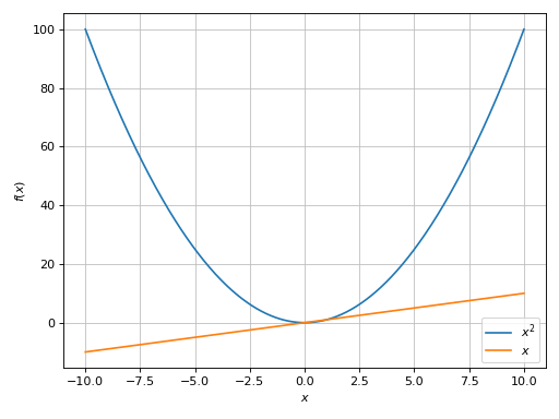
- spb.backends.base_backend.Plot.extend(self, arg)
Adds all series from another plot.
- Parameters:
- argPlot or sequence of BaseSeries
See also
Examples
Consider two Plot objects, p1 and p2. To add the second plot to the first, use the extend method, like so:
>>> from sympy import symbols
>>> from spb import plot
>>> x = symbols('x')
>>> p1 = plot(x**2, show=False)
>>> p2 = plot(x, -x, show=False)
>>> p1.extend(p2)
>>> p1
Plot object containing:
[0]: cartesian line: x**2 for x over (-10.0, 10.0)
[1]: cartesian line: x for x over (-10.0, 10.0)
[2]: cartesian line: -x for x over (-10.0, 10.0)
>>> p1.show()
(
Source code,png)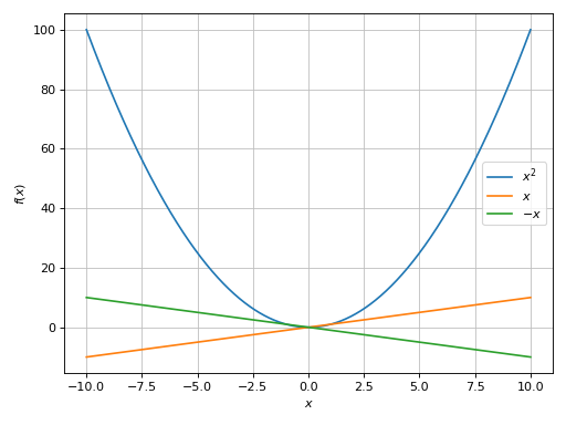
- spb.backends.base_backend.Plot.update_interactive(self, params)
Implement the logic to update the data generated by interactive-widget plots.
- Parameters:
- paramsdict
Map parameter-symbols to numeric values.
- Plot.colorloop = []
List of colors to be used in line plots or solid color surfaces.
- Plot.colormaps = []
List of color maps to render surfaces.
- Plot.cyclic_colormaps = []
List of cyclic color maps to render complex series (the phase/argument ranges over [-pi, pi]).
- Plot.fig
Returns the figure used to render/display the plots.