Vectors
NOTE:
For technical reasons, all interactive-widgets plots in this documentation
are created using Holoviz’s Panel. Often, they will ran just fine with
ipywidgets too. However, if a specific example uses the param library,
or widgets from the panel module, then users will have to modify the
params dictionary in order to make it work with ipywidgets.
Refer to Interactive module for more information.
- spb.graphics.vectors.arrow_2d(start, direction, label=None, rendering_kw=None, show_in_legend=True, **kwargs)[source]
Draw an arrow in a 2D space.
- Parameters:
- startlist, tuple, ndarray, Tuple
Coordinates of the start position, (x, y).
- directionlist, tuple, ndarray, Tuple
Componenents of the direction vector, (u, v).
- labelstr
Set the label associated to this series, which will be eventually shown on the legend or colorbar.
- rendering_kwdict
A dictionary of keyword arguments to be passed to the renderers in order to further customize the appearance of the arrows. Here are some useful links for the supported plotting libraries:
- show_in_legendbool
Toggle the visibility of the data series on the legend. Default value: True.
- paramsdict, optional
A dictionary mapping symbols to parameters. If provided, this dictionary enables the interactive-widgets plot.
When calling a plotting function, the parameter can be specified with:
a widget from the
ipywidgetsmodule.a widget from the
panelmodule.- a tuple of the form:
(default, min, max, N, tick_format, label, spacing), which will instantiate a
ipywidgets.widgets.widget_float.FloatSlideror aipywidgets.widgets.widget_float.FloatLogSlider, depending on the spacing strategy. In particular:- default, min, maxfloat
Default value, minimum value and maximum value of the slider, respectively. Must be finite numbers. The order of these 3 numbers is not important: the module will figure it out which is what.
- Nint, optional
Number of steps of the slider.
- tick_formatstr or None, optional
Provide a formatter for the tick value of the slider. Default to
".2f".
- label: str, optional
Custom text associated to the slider.
- spacingstr, optional
Specify the discretization spacing. Default to
"linear", can be changed to"log".
Notes:
parameters cannot be linked together (ie, one parameter cannot depend on another one).
If a widget returns multiple numerical values (like
panel.widgets.slider.RangeSlideroripywidgets.widgets.widget_float.FloatRangeSlider), then a corresponding number of symbols must be provided.
Here follows a couple of examples. If
imodule="panel":import panel as pn params = { a: (1, 0, 5), # slider from 0 to 5, with default value of 1 b: pn.widgets.FloatSlider(value=1, start=0, end=5), # same slider as above (c, d): pn.widgets.RangeSlider(value=(-1, 1), start=-3, end=3, step=0.1) }
Or with
imodule="ipywidgets":import ipywidgets as w params = { a: (1, 0, 5), # slider from 0 to 5, with default value of 1 b: w.FloatSlider(value=1, min=0, max=5), # same slider as above (c, d): w.FloatRangeSlider(value=(-1, 1), min=-3, max=3, step=0.1) }
When instantiating a data series directly,
paramsmust be a dictionary mapping symbols to numerical values.Let
seriesbe any data series. Thenseries.paramsreturns a dictionary mapping symbols to numerical values.- txcallable
Numerical transformation function to be applied to the data on the x-axis.
- tycallable
Numerical transformation function to be applied to the data on the y-axis.
- Returns:
- A list containing one instance of
Arrow2DSeries.
- A list containing one instance of
See also
Examples
>>> from spb import *
>>> graphics(
...     arrow_2d((0, 0), (1, 1)),
...     arrow_2d((0, 0), (-1, 1)),
...     grid=False, aspect="equal"
... )
Plot object containing:
[0]: 2D arrow from (0.0, 0.0) to (1.0, 1.0)
[1]: 2D arrow from (0.0, 0.0) to (-1.0, 1.0)
(
Source code,png)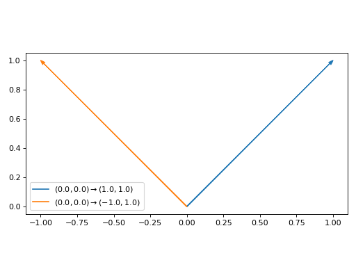
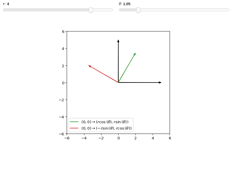
Interactive-widget plot of arrows. Refer to the interactive sub-module documentation to learn more about the
paramsdictionary.from sympy import * from spb import * r, theta = symbols("r, theta") params = { r: (4, 0, 5), theta: (pi/3, 0, 2*pi), } graphics( arrow_2d( (0, 0), (5, 0), show_in_legend=False, rendering_kw={"color": "k"}), arrow_2d( (0, 0), (0, 5), show_in_legend=False, rendering_kw={"color": "k"}), arrow_2d( (0, 0), (r * cos(theta), r * sin(theta)), params=params), arrow_2d( (0, 0), (r * cos(theta + pi/2), r * sin(theta + pi/2)), params=params), xlim=(-6, 6), ylim=(-6, 6), aspect="equal", grid=False )
- spb.graphics.vectors.arrow_3d(start, direction, label=None, rendering_kw=None, show_in_legend=True, **kwargs)[source]
Draw an arrow in a 2D space.
- Parameters:
- startlist, tuple, ndarray, Tuple
Coordinates of the start position, (x, y, z).
- directionlist, tuple, ndarray, Tuple
Componenents of the direction vector, (u, v, w).
- labelstr
Set the label associated to this series, which will be eventually shown on the legend or colorbar.
- rendering_kwdict
A dictionary of keyword arguments to be passed to the renderers in order to further customize the appearance of the arrows. Here are some useful links for the supported plotting libraries:
Matplotlib: https://matplotlib.org/stable/api/_as_gen/matplotlib.patches.FancyArrowPatch.html
K3D-Jupyter: Look at the documentation of k3d.vectors.
- show_in_legendbool
Toggle the visibility of the data series on the legend. Default value: True.
- paramsdict, optional
A dictionary mapping symbols to parameters. If provided, this dictionary enables the interactive-widgets plot.
When calling a plotting function, the parameter can be specified with:
a widget from the
ipywidgetsmodule.a widget from the
panelmodule.- a tuple of the form:
(default, min, max, N, tick_format, label, spacing), which will instantiate a
ipywidgets.widgets.widget_float.FloatSlideror aipywidgets.widgets.widget_float.FloatLogSlider, depending on the spacing strategy. In particular:- default, min, maxfloat
Default value, minimum value and maximum value of the slider, respectively. Must be finite numbers. The order of these 3 numbers is not important: the module will figure it out which is what.
- Nint, optional
Number of steps of the slider.
- tick_formatstr or None, optional
Provide a formatter for the tick value of the slider. Default to
".2f".
- label: str, optional
Custom text associated to the slider.
- spacingstr, optional
Specify the discretization spacing. Default to
"linear", can be changed to"log".
Notes:
parameters cannot be linked together (ie, one parameter cannot depend on another one).
If a widget returns multiple numerical values (like
panel.widgets.slider.RangeSlideroripywidgets.widgets.widget_float.FloatRangeSlider), then a corresponding number of symbols must be provided.
Here follows a couple of examples. If
imodule="panel":import panel as pn params = { a: (1, 0, 5), # slider from 0 to 5, with default value of 1 b: pn.widgets.FloatSlider(value=1, start=0, end=5), # same slider as above (c, d): pn.widgets.RangeSlider(value=(-1, 1), start=-3, end=3, step=0.1) }
Or with
imodule="ipywidgets":import ipywidgets as w params = { a: (1, 0, 5), # slider from 0 to 5, with default value of 1 b: w.FloatSlider(value=1, min=0, max=5), # same slider as above (c, d): w.FloatRangeSlider(value=(-1, 1), min=-3, max=3, step=0.1) }
When instantiating a data series directly,
paramsmust be a dictionary mapping symbols to numerical values.Let
seriesbe any data series. Thenseries.paramsreturns a dictionary mapping symbols to numerical values.- txcallable
Numerical transformation function to be applied to the data on the x-axis.
- tycallable
Numerical transformation function to be applied to the data on the y-axis.
- tzcallable
Numerical transformation function to be applied to the data on the z-axis.
- Returns:
- A list containing one instance of
Arrow3DSeries.
- A list containing one instance of
See also
Examples
>>> from spb import *
>>> graphics(
...     arrow_3d((0, 0, 0), (1, 0, 0)),
...     arrow_3d((0, 0, 0), (0, 1, 0)),
...     arrow_3d((0, 0, 0), (0, 0, 1), show_in_legend=False,
...              rendering_kw={
...                  "mutation_scale": 20,
...                  "arrowstyle": "-|>",
...                  "linestyle": 'dashed',
...              }),
...     xlabel="x", ylabel="y", zlabel="z")
Plot object containing:
[0]: 3D arrow from (0.0, 0.0, 0.0) to (1.0, 0.0, 0.0)
[1]: 3D arrow from (0.0, 0.0, 0.0) to (0.0, 1.0, 0.0)
[2]: 3D arrow from (0.0, 0.0, 0.0) to (0.0, 0.0, 1.0)
(
Source code,png)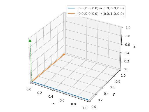
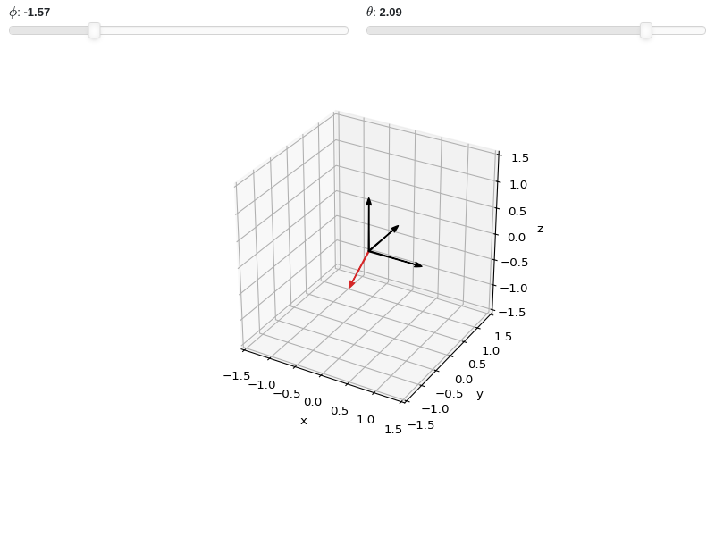
Interactive-widget plot of arrows. Refer to the interactive sub-module documentation to learn more about the
paramsdictionary.from sympy import * from spb import * phi, theta = symbols("phi, theta") r = 0.75 params = { phi: (-pi/2, -pi, pi), theta: (2*pi/3, -pi, pi), } graphics( arrow_3d((0, 0, 0), (1, 0, 0), rendering_kw={"color": "k"}, show_in_legend=False), arrow_3d((0, 0, 0), (0, 1, 0), rendering_kw={"color": "k"}, show_in_legend=False), arrow_3d((0, 0, 0), (0, 0, 1), rendering_kw={"color": "k"}, show_in_legend=False), arrow_3d( (0, 0, 0), (r*sin(theta)*cos(phi), r*sin(theta)*sin(phi), r*cos(theta)), params=params), xlabel="x", ylabel="y", zlabel="z", xlim=(-1.5, 1.5), ylim=(-1.5, 1.5), zlim=(-1.5, 1.5), aspect="equal" )
- spb.graphics.vectors.vector_field_2d(u, v=None, range_x=None, range_y=None, label=None, is_streamlines=False, quiver_kw=None, stream_kw=None, contour_kw=None, **kwargs)[source]
Plot a 2D vector field.
- Parameters:
- uVector, Expr or callable
The first component of the vector field. It can be:
A symbolic expression.
A numerical functions of 2 variables supporting vectorization.
A vector from the sympy.vector module or from the sympy.physics.mechanics module. In this case,
vcan be None and the algorithm will extract the components.
- vExpr or callable
The second component of the vector field. It can be:
A symbolic expression.
A numerical functions of 2 variables supporting vectorization.
- range_xtuple, Tuple
A 3-tuple (symb, min, max) denoting the range of the x variable. Default values: min=-10 and max=10.
- range_ytuple, Tuple
A 3-tuple (symb, min, max) denoting the range of the y variable. Default values: min=-10 and max=10.
- labelstr
Set the label associated to this series, which will be eventually shown on the legend or colorbar.
- is_streamlinesbool
If True shows the streamlines, otherwise visualize the vector field with quivers. Default value: False.
- quiver_kwdict, optional
A dictionary of keyword arguments to be passed to the renderers in order to further customize the appearance of the quivers. Here are some useful links for the supported plotting libraries:
- stream_kwdict, optional
A dictionary of keyword arguments to be passed to the renderers in order to further customize the appearance of the streamlines. Here are some useful links for the supported plotting libraries:
- contour_kwdict, optional
A dictionary of keywords/values which is passed to the backend contour function to customize the appearance. Refer to the plotting library (backend) manual for more informations.
- color_func
Define the quiver/streamlines color mapping when
use_cm=True. It can either be:A numerical function supporting vectorization. The arity must be:
f(x, y, u, v). Further,scalar=Falsemust be set in order to hide the contour plot so that a colormap is applied to quivers/streamlines.A symbolic expression having at most as many free symbols as
u, v. This only works for quivers plot.None: the default value, which will map colors according to the magnitude of the vector field.
- colorbarbool
Toggle the visibility of the colorbar associated to the current data series. Note that a colorbar is only visible if
use_cm=Trueandcolor_funcis not None. Default value: True.- force_real_evalbool
By default, numerical evaluation is performed over complex numbers, which is slower but produces correct results. However, when the symbolic expression is converted to a numerical function with lambdify, the resulting function may not like to be evaluated over complex numbers. In such cases, forcing the evaluation to be performed over real numbers might be a good choice. The plotting module should be able to detect such occurences and automatically activate this option. If that is not the case, or evaluation performance is of paramount importance, set this parameter to True, but be aware that it might produce wrong results. Default value: False.
- modules
Specify the evaluation modules to be used by lambdify. If not specified, the evaluation will be done with NumPy/SciPy.
- n1int
Number of discretization points along the x-axis to be used in the evaluation. Related parameters:
xscale. Default value: 25.- n2int
Number of discretization points along the y-axis to be used in the evaluation. Related parameters:
yscale. Default value: 25.- ncint, optional
Number of discretization points for the scalar contour plot. Default to 100.
- normalizebool
If True, the vector field will be normalized, resulting in quivers having the same length. If
use_cm=True, the backend will color the quivers by the (pre-normalized) vector field’s magnitude. Note: only quivers will be affected by this option.Default value: False.
- only_integersbool
Discretize the domain using only integer numbers. When this parameter is True, the number of discretization points is choosen by the algorithm. Default value: False.
- paramsdict, optional
A dictionary mapping symbols to parameters. If provided, this dictionary enables the interactive-widgets plot.
When calling a plotting function, the parameter can be specified with:
a widget from the
ipywidgetsmodule.a widget from the
panelmodule.- a tuple of the form:
(default, min, max, N, tick_format, label, spacing), which will instantiate a
ipywidgets.widgets.widget_float.FloatSlideror aipywidgets.widgets.widget_float.FloatLogSlider, depending on the spacing strategy. In particular:- default, min, maxfloat
Default value, minimum value and maximum value of the slider, respectively. Must be finite numbers. The order of these 3 numbers is not important: the module will figure it out which is what.
- Nint, optional
Number of steps of the slider.
- tick_formatstr or None, optional
Provide a formatter for the tick value of the slider. Default to
".2f".
- label: str, optional
Custom text associated to the slider.
- spacingstr, optional
Specify the discretization spacing. Default to
"linear", can be changed to"log".
Notes:
parameters cannot be linked together (ie, one parameter cannot depend on another one).
If a widget returns multiple numerical values (like
panel.widgets.slider.RangeSlideroripywidgets.widgets.widget_float.FloatRangeSlider), then a corresponding number of symbols must be provided.
Here follows a couple of examples. If
imodule="panel":import panel as pn params = { a: (1, 0, 5), # slider from 0 to 5, with default value of 1 b: pn.widgets.FloatSlider(value=1, start=0, end=5), # same slider as above (c, d): pn.widgets.RangeSlider(value=(-1, 1), start=-3, end=3, step=0.1) }
Or with
imodule="ipywidgets":import ipywidgets as w params = { a: (1, 0, 5), # slider from 0 to 5, with default value of 1 b: w.FloatSlider(value=1, min=0, max=5), # same slider as above (c, d): w.FloatRangeSlider(value=(-1, 1), min=-3, max=3, step=0.1) }
When instantiating a data series directly,
paramsmust be a dictionary mapping symbols to numerical values.Let
seriesbe any data series. Thenseries.paramsreturns a dictionary mapping symbols to numerical values.- rendering_kwdict
A dictionary of keyword arguments to be passed to the renderers in order to further customize the appearance of the quivers or streamlines. Here are some useful links for the supported plotting libraries:
Matplotlib:
Plotly:
2D quivers: https://plotly.com/python/quiver-plots/
2D streamlines: https://plotly.com/python/streamline-plots/
- scalarboolean, Expr, None or list or tuple of 2 elements, optional
Represents the scalar field to be plotted in the background of a 2D vector field plot. It can be:
True: plot the magnitude of the vector field. Only works when a single vector field is plotted.
False/None: do not plot any scalar field.
Expr: a symbolic expression representing the scalar field.
a numerical function of 2 variables supporting vectorization.
list/tuple: [scalar_expr, label], where the label will be shown on the colorbar. scalar_expr can be a symbolic expression or a numerical function of 2 variables supporting vectorization.
Default to True.
- show_in_legendbool
Toggle the visibility of the data series on the legend. Default value: True.
- sum_boundint
When plotting sums, the expression will be pre-processed in order to replace lower/upper bounds set to +/- infinity with this +/- numerical value. Note: the higher this number, the slower the evaluation, but the more accurate the plot. It must be: 0 ≤ sum_bound < ∞. Default value: 1000.
- txcallable
Numerical transformation function to be applied to the data on the x-axis.
- tycallable
Numerical transformation function to be applied to the data on the y-axis.
- use_cmbool
Toggle the use of a colormap. By default, some series might use a colormap to display the necessary data. Setting this attribute to False will inform the associated renderer to use solid color. Related parameters:
color_func. Default value: False.- xscalestr
Discretization strategy along the x-direction. Related parameters:
n1. Possible options: [‘linear’, ‘log’] Default value: ‘linear’.- yscalestr
Discretization strategy along the y-direction. Related parameters:
n2. Possible options: [‘linear’, ‘log’] Default value: ‘linear’.
- Returns:
- serieslist
A list containing one instance of
ContourSeries(ifscalaris set) and one instance ofVector2DSeries.
See also
Examples
>>> from sympy import symbols, sin, cos, Plane, Matrix, sqrt, latex
>>> from spb import *
>>> x, y, z = symbols('x, y, z')
Quivers plot of a 2D vector field with a contour plot in background representing the vector’s magnitude (a scalar field).
>>> graphics(
...     vector_field_2d(sin(x - y), cos(x + y), (x, -3, 3), (y, -3, 3),
...         quiver_kw=dict(color="black", scale=30, headwidth=5),
...         contour_kw={"cmap": "Blues_r", "levels": 15}),
...     grid=False, xlabel="x", ylabel="y")
Plot object containing:
[0]: contour: sqrt(sin(x - y)**2 + cos(x + y)**2) for x over (-3, 3) and y over (-3, 3)
[1]: 2D vector series: [sin(x - y), cos(x + y)] over (x, -3.0, 3.0), (y, -3.0, 3.0)
(
Source code,png)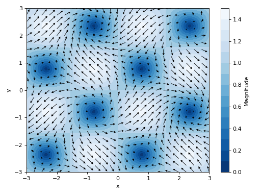
Quivers plot of a 2D vector field with no background scalar field, a custom label and normalized quiver lengths:
>>> graphics(
...     vector_field_2d(sin(x - y), cos(x + y), (x, -3, 3), (y, -3, 3),
...         label="Magnitude of $%s$" % latex([-sin(y), cos(x)]),
...         scalar=False, normalize=True,
...         quiver_kw={
...             "scale": 35, "headwidth": 4, "cmap": "gray",
...             "clim": [0, 1.6]}),
...     grid=False, xlabel="x", ylabel="y")
Plot object containing:
[0]: 2D vector series: [sin(x - y), cos(x + y)] over (x, -3.0, 3.0), (y, -3.0, 3.0)
(
Source code,png)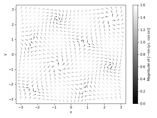
Streamlines plot of a 2D vector field with no background scalar field, and a custom label:
>>> graphics(
...     vector_field_2d(sin(x - y), cos(x + y), (x, -3, 3), (y, -3, 3),
...         streamlines=True, scalar=None,
...         stream_kw={"density": 1.5},
...         label="Magnitude of %s" % str([sin(x - y), cos(x + y)])),
...     xlabel="x", ylabel="y", grid=False)
Plot object containing:
[0]: 2D vector series: [sin(x - y), cos(x + y)] over (x, -3.0, 3.0), (y, -3.0, 3.0)
(
Source code,png)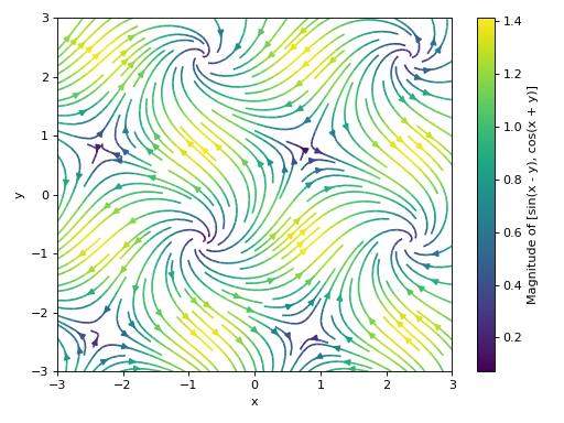
Plot multiple 2D vectors fields, setting a background scalar field to be the magnitude of the first vector. Also, apply custom rendering options to all data series.
>>> scalar_expr = sqrt((-sin(y))**2 + cos(x)**2)
>>> graphics(
...     vector_field_2d(-sin(y), cos(x), (x, -5, 5), (y, -3, 3), n=20,
...         scalar=[scalar_expr, "$%s$" % latex(scalar_expr)],
...         contour_kw={"cmap": "summer"},
...         quiver_kw={"color": "k"}),
...     vector_field_2d(2 * y, x, (x, -5, 5), (y, -3, 3), n=20,
...         scalar=False, quiver_kw={"color": "r"}, use_cm=False),
...     aspect="equal", grid=False, xlabel="x", ylabel="y")
Plot object containing:
[0]: contour: sqrt(sin(y)**2 + cos(x)**2) for x over (-5, 5) and y over (-3, 3)
[1]: 2D vector series: [-sin(y), cos(x)] over (x, -5.0, 5.0), (y, -3.0, 3.0)
[2]: 2D vector series: [2*y, x] over (x, -5.0, 5.0), (y, -3.0, 3.0)
(
Source code,png)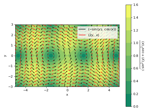
Plotting a the streamlines of a 2D vector field defined with numerical functions instead of symbolic expressions:
>>> import numpy as np
>>> f = lambda x, y: np.sin(2 * x + 2 * y)
>>> fx = lambda x, y: np.cos(f(x, y))
>>> fy = lambda x, y: np.sin(f(x, y))
>>> graphics(
...     vector_field_2d(fx, fy, ("x", -1, 1), ("y", -1, 1),
...         streamlines=True, scalar=False, use_cm=False),
...     aspect="equal", xlabel="x", ylabel="y", grid=False
... )
(
Source code,png)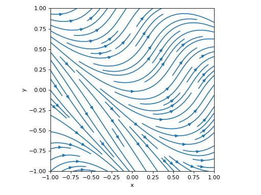
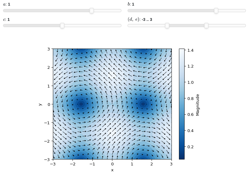
Interactive-widget 2D vector plot. Refer to the interactive sub-module documentation to learn more about the
paramsdictionary. This plot illustrates:customizing the appearance of quivers and countour.
the use of
prange(parametric plotting range).the use of the
paramsdictionary to specify sliders in their basic form: (default, min, max).the use of
panel.widgets.slider.RangeSlider, which is a 2-values widget.
from sympy import *
from spb import *
import panel as pn
x, y, a, b, c, d, e = symbols("x, y, a, b, c, d, e")
v = [-sin(a * y), cos(b * x)]
graphics(
    vector_field_2d(-sin(a * y), cos(b * x),
        prange(x, -3*c, 3*c), prange(y, d, e),
        params={
            a: (1, -2, 2), b: (1, -2, 2),
            c: (1, 0, 2),
            (d, e): pn.widgets.RangeSlider(
                value=(-3, 3), start=-9, end=9, step=0.1)
        },
        quiver_kw=dict(color="black", scale=30, headwidth=5),
        contour_kw={"cmap": "Blues_r", "levels": 15}
    ),
    grid=False, xlabel="x", ylabel="y")
- spb.graphics.vectors.vector_field_3d(u, v=None, w=None, range_x=None, range_y=None, range_z=None, label=None, is_streamlines=False, quiver_kw=None, stream_kw=None, **kwargs)[source]
Plot a 3D vector field in a cartesian coordinate system.
Note that while it is possible to define vectors in a curvilinear coordinate system (spherical, cylindrical, etc.), the vector must first be expressed in a Cartesian system. More about this in the Examples section.
- Parameters:
- uVector, Expr or callable
The first component of the vector field. It can be:
A symbolic expression.
A numerical functions of 2 variables supporting vectorization.
A vector from the sympy.vector module or from the sympy.physics.mechanics module. In this case,
v, wcan be None and the algorithm will extract the components.
- vExpr or callable
The second component of the vector field. It can be:
A symbolic expression.
A numerical functions of 2 variables supporting vectorization.
- wExpr or callable
The second component of the vector field. It can be:
A symbolic expression.
A numerical functions of 2 variables supporting vectorization.
- range_xtuple, Tuple
A 3-tuple (symb, min, max) denoting the range of the x variable. Default values: min=-10 and max=10.
- range_ytuple, Tuple
A 3-tuple (symb, min, max) denoting the range of the y variable. Default values: min=-10 and max=10.
- range_ztuple, Tuple
A 3-tuple (symb, min, max) denoting the range of the z variable. Default values: min=-10 and max=10.
- labelstr
Set the label associated to this series, which will be eventually shown on the legend or colorbar.
- is_streamlinesbool
If True shows the streamlines, otherwise visualize the vector field with quivers. Default value: False.
- quiver_kwdict, optional
A dictionary of keyword arguments to be passed to the renderers in order to further customize the appearance of the quivers. Here are some useful links for the supported plotting libraries:
- stream_kwdict, optional
A dictionary of keywords/values which is passed to the backend streamlines-plotting function to customize the appearance.
By default, the streamlines will start at the boundaries of the domain where the vectors are pointed inward. Depending on the vector field, this may results in too tight streamlines. Use the
startskeyword argument to control the generation of streamlines:starts=None: the default aforementioned behaviour.starts=dict(x=x_list, y=y_list, z=z_list): specify the starting points of the streamlines.starts=True: randomly create starting points inside the domain. In this setup we can set the number of starting point withnpoints(default value to 200).
If 3D streamlines appears to be cut short inside the specified domain, try to increase
max_prop(default value to 5000).To further customize the appearance, here are some useful links for the supported plotting libraries:
K3D-Jupyter: refers to k3d.line documentation.
- color_func
Define the quiver/streamlines color mapping when
use_cm=True. It can either be:A numerical function supporting vectorization. The arity must be
f(x, y, z, u, v, w).A symbolic expression having at most as many free symbols as
u, v, w. This only works for quivers plot.None: the default value, which will map colors according to the magnitude of the vector.
- colorbarbool
Toggle the visibility of the colorbar associated to the current data series. Note that a colorbar is only visible if
use_cm=Trueandcolor_funcis not None. Default value: True.- force_real_evalbool
By default, numerical evaluation is performed over complex numbers, which is slower but produces correct results. However, when the symbolic expression is converted to a numerical function with lambdify, the resulting function may not like to be evaluated over complex numbers. In such cases, forcing the evaluation to be performed over real numbers might be a good choice. The plotting module should be able to detect such occurences and automatically activate this option. If that is not the case, or evaluation performance is of paramount importance, set this parameter to True, but be aware that it might produce wrong results. Default value: False.
- modules
Specify the evaluation modules to be used by lambdify. If not specified, the evaluation will be done with NumPy/SciPy.
- n1int
Number of discretization points along the x-axis to be used in the evaluation. Related parameters:
xscale. Default value: 10.- n2int
Number of discretization points along the y-axis to be used in the evaluation. Related parameters:
yscale. Default value: 10.- n3int
Number of discretization points along the z-axis to be used in the evaluation. Related parameters:
zscale. Default value: 10.- normalizebool
If True, the vector field will be normalized, resulting in quivers having the same length. If
use_cm=True, the backend will color the quivers by the (pre-normalized) vector field’s magnitude. Note: only quivers will be affected by this option.Default value: False.
- only_integersbool
Discretize the domain using only integer numbers. When this parameter is True, the number of discretization points is choosen by the algorithm. Default value: False.
- paramsdict, optional
A dictionary mapping symbols to parameters. If provided, this dictionary enables the interactive-widgets plot.
When calling a plotting function, the parameter can be specified with:
a widget from the
ipywidgetsmodule.a widget from the
panelmodule.- a tuple of the form:
(default, min, max, N, tick_format, label, spacing), which will instantiate a
ipywidgets.widgets.widget_float.FloatSlideror aipywidgets.widgets.widget_float.FloatLogSlider, depending on the spacing strategy. In particular:- default, min, maxfloat
Default value, minimum value and maximum value of the slider, respectively. Must be finite numbers. The order of these 3 numbers is not important: the module will figure it out which is what.
- Nint, optional
Number of steps of the slider.
- tick_formatstr or None, optional
Provide a formatter for the tick value of the slider. Default to
".2f".
- label: str, optional
Custom text associated to the slider.
- spacingstr, optional
Specify the discretization spacing. Default to
"linear", can be changed to"log".
Notes:
parameters cannot be linked together (ie, one parameter cannot depend on another one).
If a widget returns multiple numerical values (like
panel.widgets.slider.RangeSlideroripywidgets.widgets.widget_float.FloatRangeSlider), then a corresponding number of symbols must be provided.
Here follows a couple of examples. If
imodule="panel":import panel as pn params = { a: (1, 0, 5), # slider from 0 to 5, with default value of 1 b: pn.widgets.FloatSlider(value=1, start=0, end=5), # same slider as above (c, d): pn.widgets.RangeSlider(value=(-1, 1), start=-3, end=3, step=0.1) }
Or with
imodule="ipywidgets":import ipywidgets as w params = { a: (1, 0, 5), # slider from 0 to 5, with default value of 1 b: w.FloatSlider(value=1, min=0, max=5), # same slider as above (c, d): w.FloatRangeSlider(value=(-1, 1), min=-3, max=3, step=0.1) }
When instantiating a data series directly,
paramsmust be a dictionary mapping symbols to numerical values.Let
seriesbe any data series. Thenseries.paramsreturns a dictionary mapping symbols to numerical values.- rendering_kwdict
A dictionary of keyword arguments to be passed to the renderers in order to further customize the appearance of the quivers or streamlines. Here are some useful links for the supported plotting libraries:
Matplotlib:
Plotly:
3D cones: https://plotly.com/python/cone-plot/
3D streamlines: https://plotly.com/python/streamtube-plot/
K3D-Jupyter:
for quiver plots, the keys can be:
scale: a float number acting as a scale multiplier. Default to 1.
pivot: indicates the part of the arrow that is anchored to the X, Y, Z grid. It can be
"tail", "mid", "middle", "tip". Defaul to"mid".color: set a solid color by specifying an integer color, or a colormap by specifying one of k3d’s colormaps. If this key is not provided, a default color or colormap is used, depending on the value of
use_cm.
for streamline plots, refers to k3d.line documentation.
- show_in_legendbool
Toggle the visibility of the data series on the legend. Default value: True.
- slicePlane, list, Expr, optional
Plot the 3D vector field over the provided slice. It can be:
a Plane object from sympy.geometry module.
a list of planes.
an instance of
SurfaceOver2DRangeSeriesorParametricSurfaceSeries.a symbolic expression representing a surface of two variables.
The number of discretization points will be n1, n2, n3. Note that:
only quivers plots are supported with slices. Streamlines plots are unaffected.
n3 will only be used with planes parallel to xz or yz.
n1, n2, n3 doesn’t affect the slice if it is an instance of
SurfaceOver2DRangeSeriesorParametricSurfaceSeries.
- sum_boundint
When plotting sums, the expression will be pre-processed in order to replace lower/upper bounds set to +/- infinity with this +/- numerical value. Note: the higher this number, the slower the evaluation, but the more accurate the plot. It must be: 0 ≤ sum_bound < ∞. Default value: 1000.
- txcallable
Numerical transformation function to be applied to the data on the x-axis.
- tycallable
Numerical transformation function to be applied to the data on the y-axis.
- tzcallable
Numerical transformation function to be applied to the data on the z-axis.
- use_cmbool
Toggle the use of a colormap. By default, some series might use a colormap to display the necessary data. Setting this attribute to False will inform the associated renderer to use solid color. Related parameters:
color_func. Default value: False.- xscalestr
Discretization strategy along the x-direction. Related parameters:
n1. Possible options: [‘linear’, ‘log’] Default value: ‘linear’.- yscalestr
Discretization strategy along the y-direction. Related parameters:
n2. Possible options: [‘linear’, ‘log’] Default value: ‘linear’.- zscalestr
Discretization strategy along the z-direction. Related parameters:
n3. Possible options: [‘linear’, ‘log’] Default value: ‘linear’.
- Returns:
- serieslist
If
sliceis not set, the function returns a list containing one instance ofVector3DSeries. Conversely, it returns a list containing instances ofSliceVector3DSeries.
See also
Examples
Plot a 3D vector field defined in a Cartesian coordinate system:
from sympy import *
from spb import *
var("x:z")
graphics(
    vector_field_3d(z, y, x, (x, -10, 10), (y, -10, 10), (z, -10, 10),
        n=8, quiver_kw={"scale": 0.5, "line_width": 0.1, "head_size": 10}),
    backend=KB, xlabel="x", ylabel="y", zlabel="z")
3D vector field over 3 orthogonal slice planes.
from sympy import *
from spb import *
var("x:z")
graphics(
    vector_field_3d(z, y, x, (x, -10, 10), (y, -10, 10), (z, -10, 10),
        n=8, use_cm=False,
        quiver_kw={"scale": 0.25, "line_width": 0.1, "head_size": 10},
        slice=[
            Plane((-10, 0, 0), (1, 0, 0)),
            Plane((0, 10, 0), (0, 2, 0)),
            Plane((0, 0, -10), (0, 0, 1))]
    ),
    backend=KB, grid=False, xlabel="x", ylabel="y", zlabel="z",)
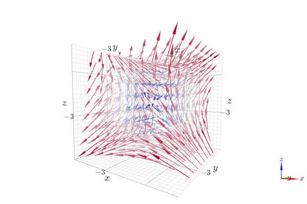
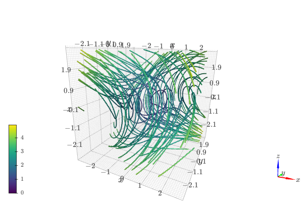
3D streamlines starting at a 400 random points:
from sympy import *
from spb import *
import k3d
var("x:z")
graphics(
    vector_field_3d(z, -x, y, (x, -3, 3), (y, -3, 3), (z, -3, 3),
        n=40, streamlines=True,
        stream_kw=dict(
            starts=True,
            npoints=400,
            width=0.025,
            color_map=k3d.colormaps.matplotlib_color_maps.viridis
        )
    ),
    backend=KB, xlabel="x", ylabel="y", zlabel="z")
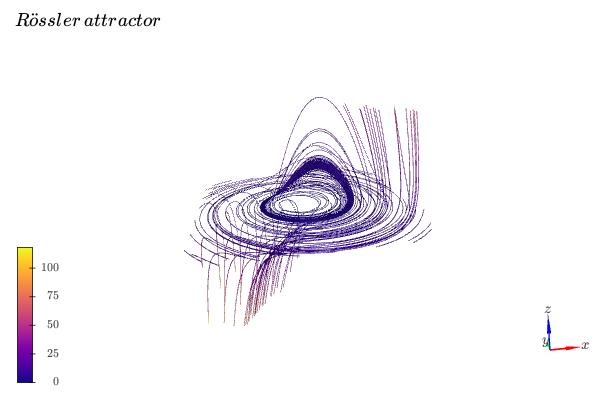
3D vector streamlines starting at the XY plane. Note that the number of discretization points of the plane controls the numbers of streamlines.
from sympy import *
from spb import *
import k3d
var("x:z")
u = -y - z
v = x + y / 5
w = S(1) / 5 + (x - S(5) / 2) * z
s = 10 # length of the cubic discretization volume
# create an XY plane with n discretization points along each direction
n = 8
p = plane(
    Plane((0, 0, 0), (0, 0, 1)), (x, -s, s), (y, -s, s), (z, -s, s),
    n1=n, n2=n)[0]
xx, yy, zz = p.get_data()
graphics(
    vector_field_3d(
        u, v, w, (x, -s, s), (y, -s, s), (z, -s, s),
        n=40, streamlines=True,
        stream_kw=dict(
            starts=dict(x=xx, y=yy, z=zz),
            width=0.025,
            color_map=k3d.colormaps.matplotlib_color_maps.plasma
        )),
    title="Rössler \, attractor", xlabel="x", ylabel="y", zlabel="z",
    backend=KB, grid=False)
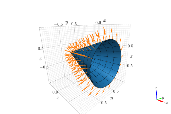
Visually verify the normal vector to a circular cone surface. The following steps are executed:
compute the normal vector to a circular cone surface. This will be the vector field to be plotted.
create a data series representing the cone surface for visualization purposes (use high number of discretization points).
create a data series representing the cone surface that will be used to slice the vector field (use a low number of discretization points).
create a data series for the normal vector, and assign step 3 to the
slicekeyword.Assemble the
graphicscommand and get a nice visualization.
from sympy import tan, cos, sin, pi, symbols
from spb import *
from sympy.vector import CoordSys3D, gradient

u, v = symbols("u, v")
N = CoordSys3D("N")
i, j, k = N.base_vectors()
xn, yn, zn = N.base_scalars()

t = 0.35    # half-cone angle in radians
expr = -xn**2 * tan(t)**2 + yn**2 + zn**2    # cone surface equation
g = gradient(expr)
n = g / g.magnitude()    # unit normal vector
n1, n2 = 10, 20 # number of discretization points for the vector field

# cone surface to discretize vector field (low numb of discret points)
cone_discr = surface_parametric(
    u / tan(t), u * cos(v), u * sin(v), (u, 0, 1), (v, 0 , 2*pi),
    n1=n1, n2=n2)[0]
graphics(
    surface_parametric(
        u / tan(t), u * cos(v), u * sin(v), (u, 0, 1), (v, 0 , 2*pi),
        rendering_kw={"opacity": 1}, wireframe=True,
        wf_n1=n1, wf_n2=n2, wf_rendering_kw={"width": 0.004}),
    vector_field_3d(
        n, range_x=(xn, -5, 5), range_y=(yn, -5, 5), range_z=(zn, -5, 5),
        use_cm=False, slice=cone_discr,
        quiver_kw={"scale": 0.5, "pivot": "tail"}
    ),
    backend=KB)
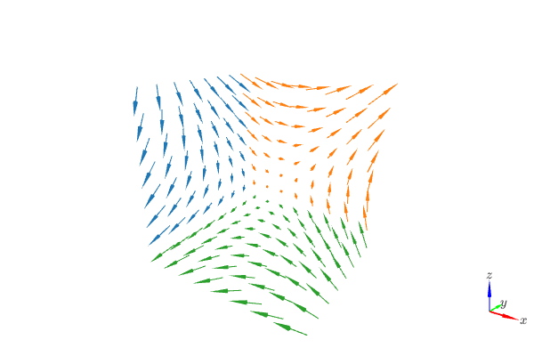
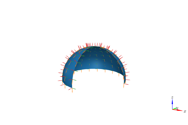
Compute the normal vector and tangent vectors to a sphere using a spherical coordinate system. Then, convert them to cartesian coordinates for plotting. The conversion is performed with the
expressfunction exposed by this module, which supports curvilinear to cartesian (and viceversa) transformations:from sympy import * from spb import * from spb.graphics.vector_transforms import express from sympy.vector import CoordSys3D C = CoordSys3D("C") S = C.create_new("S", transformation="spherical") x, y, z = C.base_scalars() r, theta, phi = S.base_scalars() # position vector for a point on the surface of a sphere of radius r sphere = r * S.i # get the parametric equation for a sphere parameterization = express(sphere, C).to_matrix(C).subs(r, 7) # normal and tangents to the sphere expressed in the cartesian frame, # using spherical variables n = express(sphere, C).normalize().simplify() t_theta = n.diff(theta).normalize().simplify() t_phi = n.diff(phi).normalize().simplify() # normal and tangents to the sphere expressed in the cartesian frame, # using cartesian variables d = {k: v for k, v in zip([r, theta, phi], S.transformation_from_parent())} n = n.subs(d) t_theta = t_theta.subs(d) t_phi = t_phi.subs(d) phi_max = 3 * pi / 2 theta_max = pi / 2 sphere_series = surface_parametric( *parameterization, (phi, 0, phi_max), (theta, 0, theta_max)) locations_for_vectors = surface_parametric( *parameterization, (phi, 0, phi_max), (theta, 0, theta_max), n1=15, n2=8)[0] quiver_kw=dict(pivot="tail", head_size=2, line_width=0.03) common_kws = dict( # NOTE: dummy values for ranges. The important thing is # to order them appropriately. For example, variable x must go # on range_x, etc. range_x=(x, -1, 1), range_y=(y, -1, 1), range_z=(z, -1, 1), slice=locations_for_vectors, use_cm=False, quiver_kw=quiver_kw ) graphics( sphere_series[0], vector_field_3d(t_theta, **common_kws), vector_field_3d(t_phi, **common_kws), vector_field_3d(n, **common_kws), grid=False, backend=KB )