Complex Analysis

NOTE: For technical reasons, all interactive-widgets plots in this documentation are created using Holoviz’s Panel. Often, they will ran just fine with ipywidgets too. However, if a specific example uses the param library, or widgets from the panel module, then users will have to modify the params dictionary in order to make it work with ipywidgets. Refer to Interactive module for more information.

spb.graphics.complex_analysis.complex_points(*numbers, label='', rendering_kw=None, is_scatter=True, **kwargs)

Plot complex points.

Parameters:

numbers

Complex number, or a list of complex numbers.

labelstr

Set the label associated to this series, which will be eventually shown on the legend or colorbar.

rendering_kwdict

A dictionary of keyword arguments to be passed to the renderers in order to further customize the appearance of the line. Here are some useful links for the supported plotting libraries:

• Matplotlib:

  • for solid lines: https://matplotlib.org/stable/api/_as_gen/matplotlib.pyplot.plot.html

  • for colormap-based lines: https://matplotlib.org/stable/api/collections_api.html#matplotlib.collections.LineCollection

  • for scatters: https://matplotlib.org/stable/api/_as_gen/matplotlib.pyplot.scatter.html

• Bokeh:

  • for solid lines: https://docs.bokeh.org/en/latest/docs/reference/plotting.html#bokeh.plotting.Figure.line

  • for scatter: https://docs.bokeh.org/en/latest/docs/reference/plotting/figure.html#bokeh.plotting.Figure.scatter

• Plotly: https://plotly.com/python/line-and-scatter/

is_scatterbool

If True it represent a scatter plot, otherwise a continuous line. Default value: False.

color_funccallable

A color function to be applied to the numerical data. It can be:

• None: no color function.

• callable: a function accepting two arguments, the real and imaginary parts of the complex coordinates, and returning numerical data.

colorbarbool

Toggle the visibility of the colorbar associated to the current data series. Note that a colorbar is only visible if use_cm=True and color_func is not None. Default value: True.

colorbar_ticks_formattertick_formatter_multiples_of

An object of type tick_formatter_multiples_of which will be used to place tick values on the colorbar at each multiple of a specified quantity. This only works when use_cm=True.

is_filledbool

Whether scatter’s markers are filled or void. Default value: True.

line_color

For back-compatibility with old sympy.plotting. Use rendering_kw in order to fully customize the appearance of the line/scatter.

paramsdict, optional

A dictionary mapping symbols to parameters. If provided, this dictionary enables the interactive-widgets plot.

When calling a plotting function, the parameter can be specified with:

• a widget from the ipywidgets module.

• a widget from the panel module.

• a tuple of the form:

  (default, min, max, N, tick_format, label, spacing), which will instantiate a ipywidgets.widgets.widget_float.FloatSlider or a ipywidgets.widgets.widget_float.FloatLogSlider, depending on the spacing strategy. In particular:

  • default, min, maxfloat

    Default value, minimum value and maximum value of the slider, respectively. Must be finite numbers. The order of these 3 numbers is not important: the module will figure it out which is what.

  • Nint, optional

    Number of steps of the slider.

  • tick_formatstr or None, optional

    Provide a formatter for the tick value of the slider. Default to ".2f".

  • label: str, optional

    Custom text associated to the slider.

  • spacingstr, optional

    Specify the discretization spacing. Default to "linear", can be changed to "log".

Notes:

1. parameters cannot be linked together (ie, one parameter cannot depend on another one).

2. If a widget returns multiple numerical values (like panel.widgets.slider.RangeSlider or ipywidgets.widgets.widget_float.FloatRangeSlider), then a corresponding number of symbols must be provided.

Here follows a couple of examples. If imodule="panel":

import panel as pn
params = {
    a: (1, 0, 5), # slider from 0 to 5, with default value of 1
    b: pn.widgets.FloatSlider(value=1, start=0, end=5), # same slider as above
    (c, d): pn.widgets.RangeSlider(value=(-1, 1), start=-3, end=3, step=0.1)
}

Or with imodule="ipywidgets":

import ipywidgets as w
params = {
    a: (1, 0, 5), # slider from 0 to 5, with default value of 1
    b: w.FloatSlider(value=1, min=0, max=5), # same slider as above
    (c, d): w.FloatRangeSlider(value=(-1, 1), min=-3, max=3, step=0.1)
}

When instantiating a data series directly, params must be a dictionary mapping symbols to numerical values.

Let series be any data series. Then series.params returns a dictionary mapping symbols to numerical values.

show_in_legendbool

Toggle the visibility of the data series on the legend. Default value: True.

txcallable

Numerical transformation function to be applied to the data on the x-axis.

tycallable

Numerical transformation function to be applied to the data on the y-axis.

use_cmbool

Toggle the use of a colormap. By default, some series might use a colormap to display the necessary data. Setting this attribute to False will inform the associated renderer to use solid color. Related parameters: color_func. Default value: False.

Returns:

serieslist

A list containing an instance of ComplexPointSeries.

Examples

>>> from sympy import I, symbols, exp, sqrt, cos, sin, pi, gamma
>>> from spb import *
>>> x, y, z = symbols('x, y, z')

(Source code)

Plot individual complex points:

>>> graphics(complex_points(3 + 2 * I, 4 * I, 2))
Plot object containing:
[0]: complex points: (3 + 2*I, 4*I, 2)

(Source code, png)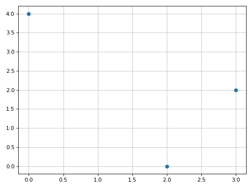

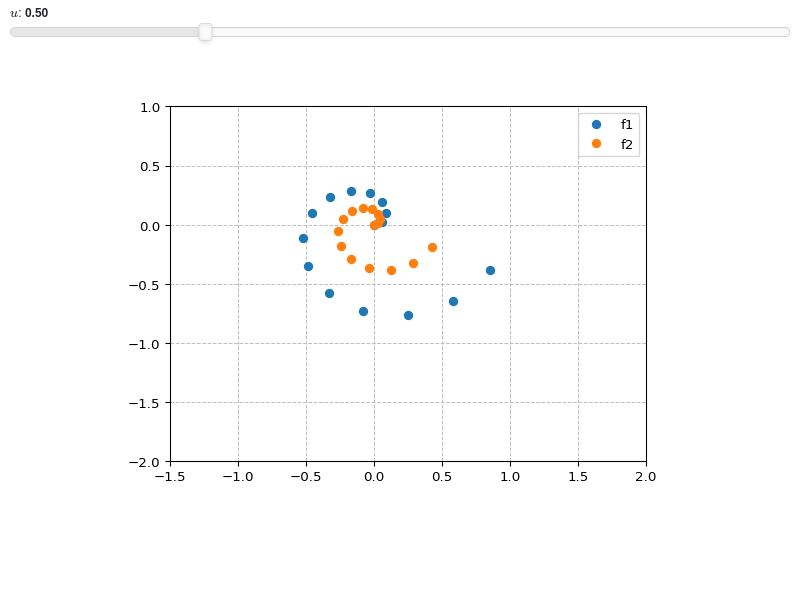
Plot two lists of complex points and assign to them custom labels:

>>> expr1 = z * exp(2 * pi * I * z)
>>> expr2 = 2 * expr1
>>> n = 15
>>> l1 = [expr1.subs(z, t / n) for t in range(n)]
>>> l2 = [expr2.subs(z, t / n) for t in range(n)]
>>> graphics(
...     complex_points(l1, label="f1"),
...     complex_points(l2, label="f2"), legend=True)
Plot object containing:
[0]: complex points: (0.0, 0.0666666666666667*exp(0.133333333333333*I*pi), 0.133333333333333*exp(0.266666666666667*I*pi), 0.2*exp(0.4*I*pi), 0.266666666666667*exp(0.533333333333333*I*pi), 0.333333333333333*exp(0.666666666666667*I*pi), 0.4*exp(0.8*I*pi), 0.466666666666667*exp(0.933333333333333*I*pi), 0.533333333333333*exp(1.06666666666667*I*pi), 0.6*exp(1.2*I*pi), 0.666666666666667*exp(1.33333333333333*I*pi), 0.733333333333333*exp(1.46666666666667*I*pi), 0.8*exp(1.6*I*pi), 0.866666666666667*exp(1.73333333333333*I*pi), 0.933333333333333*exp(1.86666666666667*I*pi))
[1]: complex points: (0, 0.133333333333333*exp(0.133333333333333*I*pi), 0.266666666666667*exp(0.266666666666667*I*pi), 0.4*exp(0.4*I*pi), 0.533333333333333*exp(0.533333333333333*I*pi), 0.666666666666667*exp(0.666666666666667*I*pi), 0.8*exp(0.8*I*pi), 0.933333333333333*exp(0.933333333333333*I*pi), 1.06666666666667*exp(1.06666666666667*I*pi), 1.2*exp(1.2*I*pi), 1.33333333333333*exp(1.33333333333333*I*pi), 1.46666666666667*exp(1.46666666666667*I*pi), 1.6*exp(1.6*I*pi), 1.73333333333333*exp(1.73333333333333*I*pi), 1.86666666666667*exp(1.86666666666667*I*pi))

(Source code, png)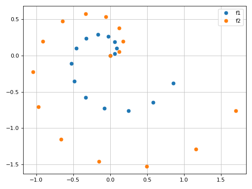

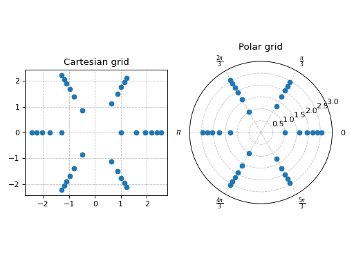
Plot the solutions of sin(z**3 - 1) = 0. Here we see that complex_points works fine when plotting over a cartesian grid, but if we need to plot complex points in polar form, then list_2d must be used instead. Note the use of a custom tick formatter in the polar plot:

>>> from sympy import Tuple, solve, arg
>>> n = symbols("n")
>>> expr = z**3 - 1
>>> eq = expr - n * pi
>>> sol = Tuple(*solve(eq, z))
>>> points = []
>>> n_lim = 5
>>> for n_val in range(-n_lim, n_lim+1):
...     points.extend(sol.subs(n, n_val))
>>>
>>> r = [complex(abs(p)).real for p in points]
>>> t = [arg(p) for p in points]
>>> p1 = graphics(
...     complex_points(points),
...     aspect="equal", title="Cartesian grid", show=False
... )
>>> p2 = graphics(
...     list_2d(t, r, is_point=True),
...     x_ticks_formatter=multiples_of_pi_over_3(),
...     title="Polar grid", ylim=(0, 3),
...     aspect="equal", polar_axis=True, show=False
... )
>>> plotgrid(p1, p2, nr=1)       

(Source code, png)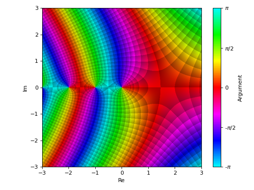

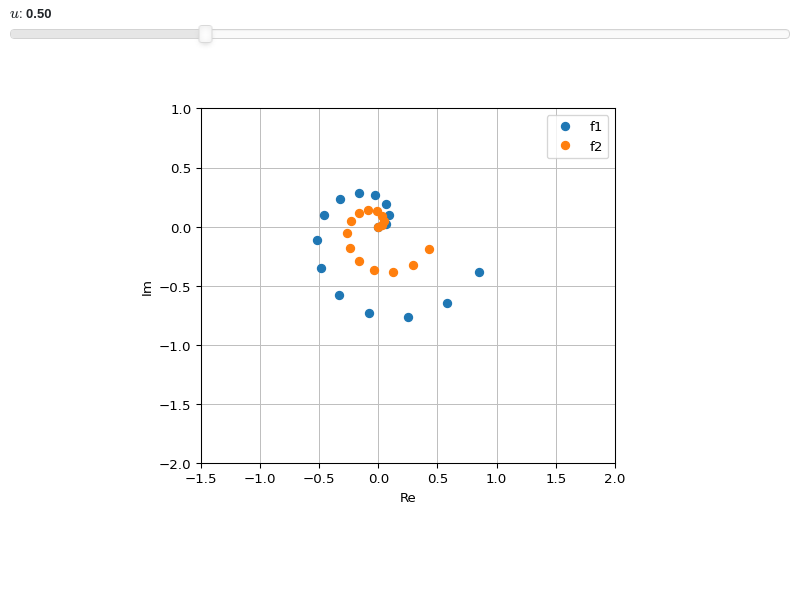
Interactive-widget plot. Refer to the interactive sub-module documentation to learn more about the params dictionary.

from sympy import *
from spb import *
z, u = symbols("z u")
expr1 = z * exp(2 * pi * I * z)
expr2 = u * expr1
n = 15
l1 = [expr1.subs(z, t / n) for t in range(n)]
l2 = [expr2.subs(z, t / n) for t in range(n)]
params = {u: (0.5, 0, 2)}
graphics(
    complex_points(l1, label="f1", params=params),
    complex_points(l2, label="f2", params=params),
    legend=True, xlim=(-1.5, 2), ylim=(-2, 1))

(Source code, small.png)

spb.graphics.complex_analysis.line_abs_arg_colored(expr, range_x=None, label=None, rendering_kw=None, **kwargs)

Plot the absolute value of a complex function f(x) colored by its argument, with x in Reals.

Parameters:

expr

It can either be a symbolic expression representing the function of one variable to be plotted, or a numerical function of one variable, supporting vectorization. In the latter case the following keyword arguments are not supported: params, sum_bound.

range_xtuple, Tuple

A 3-tuple (symb, min, max) denoting the range of the x variable. Default values: min=-10 and max=10.

labelstr

Set the label associated to this series, which will be eventually shown on the legend or colorbar.

rendering_kwdict

A dictionary of keyword arguments to be passed to the renderers in order to further customize the appearance of the line. Here are some useful links for the supported plotting libraries:

• Matplotlib:

  • for solid lines: https://matplotlib.org/stable/api/_as_gen/matplotlib.pyplot.plot.html

  • for colormap-based lines: https://matplotlib.org/stable/api/collections_api.html#matplotlib.collections.LineCollection

  • for scatters: https://matplotlib.org/stable/api/_as_gen/matplotlib.pyplot.scatter.html

• Bokeh:

  • for solid lines: https://docs.bokeh.org/en/latest/docs/reference/plotting.html#bokeh.plotting.Figure.line

  • for scatter: https://docs.bokeh.org/en/latest/docs/reference/plotting/figure.html#bokeh.plotting.Figure.scatter

• Plotly: https://plotly.com/python/line-and-scatter/

color_func

A color function to be applied to the numerical data. It can be:

• A numerical function of 2 variables, x, y (the points computed by the internal algorithm) supporting vectorization.

• A symbolic expression having at most as many free symbols as expr.

• None: the default value (no color mapping).

colorbarbool

Toggle the visibility of the colorbar associated to the current data series. Note that a colorbar is only visible if use_cm=True and color_func is not None. Default value: True.

colorbar_ticks_formattertick_formatter_multiples_of

An object of type tick_formatter_multiples_of which will be used to place tick values on the colorbar at each multiple of a specified quantity. This only works when use_cm=True.

detect_polesbool, str

Chose whether to detect and correctly plot the roots of the denominator. There are two algorithms at work:

1. based on the gradient of the numerical data, it introduces NaN values at locations where the steepness is greater than some threshold. This splits the line into multiple segments. To improve detection, increase the number of discretization points n and/or change the value of eps. This algorithm can be used to visualize jump discontinuities as well as essential discontinuities.

2. a symbolic approach based on the continuous_domain function from the sympy.calculus.util module, which computes the locations of essential discontinuities. If any are found, vertical lines will be shown.

Possible options:

• False: No poles detection

• True: Poles detection with the numerical algorithm

• ‘symbolic’: Poles detection with numerical and symbolic algorithms

Default value: False.

epsfloat

An arbitrary small value used by the detect_poles numerical algorithm. Before changing this value, it is recommended to increase the number of discretization points. Related parameters: detect_poles. It must be: 0 ≤ eps < ∞. Default value: 0.01.

excludelist

List of x-coordinates to be excluded from evaluation. In practice, it introduces discontinuities in the resulting line.

force_real_evalbool

By default, numerical evaluation is performed over complex numbers, which is slower but produces correct results. However, when the symbolic expression is converted to a numerical function with lambdify, the resulting function may not like to be evaluated over complex numbers. In such cases, forcing the evaluation to be performed over real numbers might be a good choice. The plotting module should be able to detect such occurences and automatically activate this option. If that is not the case, or evaluation performance is of paramount importance, set this parameter to True, but be aware that it might produce wrong results. Default value: False.

is_filledbool

Whether scatter’s markers are filled or void. Default value: True.

is_scatterbool

If True it represent a scatter plot, otherwise a continuous line. Default value: False.

line_color

For back-compatibility with old sympy.plotting. Use rendering_kw in order to fully customize the appearance of the line/scatter.

modules

Specify the evaluation modules to be used by lambdify. If not specified, the evaluation will be done with NumPy/SciPy.

n1int

Number of discretization points along the parameter to be used in the numerical evaluation. An alias of this parameter is n. Related parameters: xscale. It must be: 2 ≤ n1 < ∞. Default value: 1000.

only_integersbool

Discretize the domain using only integer numbers. When this parameter is True, the number of discretization points is choosen by the algorithm. Default value: False.

paramsdict, optional

A dictionary mapping symbols to parameters. If provided, this dictionary enables the interactive-widgets plot.

When calling a plotting function, the parameter can be specified with:

• a widget from the ipywidgets module.

• a widget from the panel module.

• a tuple of the form:

  (default, min, max, N, tick_format, label, spacing), which will instantiate a ipywidgets.widgets.widget_float.FloatSlider or a ipywidgets.widgets.widget_float.FloatLogSlider, depending on the spacing strategy. In particular:

  • default, min, maxfloat

    Default value, minimum value and maximum value of the slider, respectively. Must be finite numbers. The order of these 3 numbers is not important: the module will figure it out which is what.

  • Nint, optional

    Number of steps of the slider.

  • tick_formatstr or None, optional

    Provide a formatter for the tick value of the slider. Default to ".2f".

  • label: str, optional

    Custom text associated to the slider.

  • spacingstr, optional

    Specify the discretization spacing. Default to "linear", can be changed to "log".

Notes:

1. parameters cannot be linked together (ie, one parameter cannot depend on another one).

2. If a widget returns multiple numerical values (like panel.widgets.slider.RangeSlider or ipywidgets.widgets.widget_float.FloatRangeSlider), then a corresponding number of symbols must be provided.

Here follows a couple of examples. If imodule="panel":

import panel as pn
params = {
    a: (1, 0, 5), # slider from 0 to 5, with default value of 1
    b: pn.widgets.FloatSlider(value=1, start=0, end=5), # same slider as above
    (c, d): pn.widgets.RangeSlider(value=(-1, 1), start=-3, end=3, step=0.1)
}

Or with imodule="ipywidgets":

import ipywidgets as w
params = {
    a: (1, 0, 5), # slider from 0 to 5, with default value of 1
    b: w.FloatSlider(value=1, min=0, max=5), # same slider as above
    (c, d): w.FloatRangeSlider(value=(-1, 1), min=-3, max=3, step=0.1)
}

When instantiating a data series directly, params must be a dictionary mapping symbols to numerical values.

Let series be any data series. Then series.params returns a dictionary mapping symbols to numerical values.

poles_locationslist

When detect_poles="symbolic", stores the location of the computed poles (essential discontinuities) so that they can be appropriately rendered.

poles_rendering_kwdict

Rendering kw used to customize the appearance of vertical lines representing essential discontinuities. Related parameters: poles_locations.

show_in_legendbool

Toggle the visibility of the data series on the legend. Default value: True.

stepsNoneType, bool, str

If set, it connects consecutive points with steps rather than straight segments. Possible options: [‘pre’, ‘post’, ‘mid’, True, False, None] Default value: False.

sum_boundint

When plotting sums, the expression will be pre-processed in order to replace lower/upper bounds set to +/- infinity with this +/- numerical value. Note: the higher this number, the slower the evaluation, but the more accurate the plot. It must be: 0 ≤ sum_bound < ∞. Default value: 1000.

txcallable

Numerical transformation function to be applied to the data on the x-axis.

tycallable

Numerical transformation function to be applied to the data on the y-axis.

unwrapbool, dict

Whether to use numpy.unwrap() on the computed coordinates in order to get rid of discontinuities. It can be:

• False: do not use np.unwrap().

• True: use np.unwrap() with default keyword arguments.

• dictionary of keyword arguments passed to np.unwrap().

use_cmbool

Toggle the use of a colormap. By default, some series might use a colormap to display the necessary data. Setting this attribute to False will inform the associated renderer to use solid color. Related parameters: color_func. Default value: False.

xscalestr

Discretization strategy along the x-direction. Related parameters: n1. Possible options: [‘linear’, ‘log’] Default value: ‘linear’.

Returns:

serieslist

A list containing an instance of AbsArgLineSeries.

See also

spb.graphics.functions_2d.line, line_abs_arg, line_real_imag

domain_coloring

Examples

>>> from sympy import I, symbols, cos, sin, pi
>>> from spb import *
>>> x = symbols('x')

(Source code)

Plot the modulus of a complex function colored by its magnitude:

>>> graphics(
...     line_abs_arg_colored(cos(x) + sin(I * x), (x, -2, 2),
...         label="f"))
Plot object containing:
[0]: cartesian abs-arg line: cos(x) + I*sinh(x) for x over (-2, 2)

(Source code, png)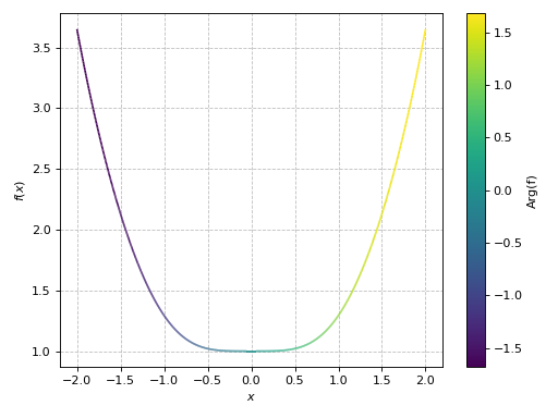

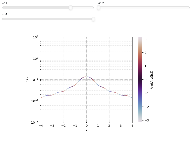
Interactive-widget plot of a Fourier Transform. Refer to the interactive sub-module documentation to learn more about the params dictionary. This plot illustrates:

• the use of prange (parametric plotting range).

• for line_abs_arg_colored, symbols going into prange must be real.

• the use of the params dictionary to specify sliders in their basic form: (default, min, max).

from sympy import *
from spb import *
x, k, a, b = symbols("x, k, a, b")
c = symbols("c", real=True)
f = exp(-x**2) * (Heaviside(x + a) - Heaviside(x - b))
fs = fourier_transform(f, x, k)
graphics(
    line_abs_arg_colored(fs, prange(k, -c, c),
        params={a: (1, -2, 2), b: (-2, -2, 2), c: (4, 0.5, 4)},
        label="Arg(fs)"),
    xlabel="k", yscale="log", ylim=(1e-03, 10))

(Source code, small.png)

spb.graphics.complex_analysis.line_abs_arg(expr, range_x=None, label=None, rendering_kw=None, abs=True, arg=True, **kwargs)

Plot the absolute value and/or the argument of a complex function f(x) with x in Reals.

Parameters:

expr

It can either be a symbolic expression representing the function of one variable to be plotted, or a numerical function of one variable, supporting vectorization. In the latter case the following keyword arguments are not supported: params, sum_bound.

range_xtuple, Tuple

A 3-tuple (symb, min, max) denoting the range of the x variable. Default values: min=-10 and max=10.

labelstr

Set the label associated to this series, which will be eventually shown on the legend or colorbar.

rendering_kwdict

A dictionary of keyword arguments to be passed to the renderers in order to further customize the appearance of the line. Here are some useful links for the supported plotting libraries:

• Matplotlib:

  • for solid lines: https://matplotlib.org/stable/api/_as_gen/matplotlib.pyplot.plot.html

  • for colormap-based lines: https://matplotlib.org/stable/api/collections_api.html#matplotlib.collections.LineCollection

  • for scatters: https://matplotlib.org/stable/api/_as_gen/matplotlib.pyplot.scatter.html

• Bokeh:

  • for solid lines: https://docs.bokeh.org/en/latest/docs/reference/plotting.html#bokeh.plotting.Figure.line

  • for scatter: https://docs.bokeh.org/en/latest/docs/reference/plotting/figure.html#bokeh.plotting.Figure.scatter

• Plotly: https://plotly.com/python/line-and-scatter/

color_func

A color function to be applied to the numerical data. It can be:

• A numerical function of 2 variables, x, y (the points computed by the internal algorithm) supporting vectorization.

• A symbolic expression having at most as many free symbols as expr.

• None: the default value (no color mapping).

colorbarbool

Toggle the visibility of the colorbar associated to the current data series. Note that a colorbar is only visible if use_cm=True and color_func is not None. Default value: True.

colorbar_ticks_formattertick_formatter_multiples_of

An object of type tick_formatter_multiples_of which will be used to place tick values on the colorbar at each multiple of a specified quantity. This only works when use_cm=True.

detect_polesbool, str

Chose whether to detect and correctly plot the roots of the denominator. There are two algorithms at work:

1. based on the gradient of the numerical data, it introduces NaN values at locations where the steepness is greater than some threshold. This splits the line into multiple segments. To improve detection, increase the number of discretization points n and/or change the value of eps. This algorithm can be used to visualize jump discontinuities as well as essential discontinuities.

2. a symbolic approach based on the continuous_domain function from the sympy.calculus.util module, which computes the locations of essential discontinuities. If any are found, vertical lines will be shown.

Possible options:

• False: No poles detection

• True: Poles detection with the numerical algorithm

• ‘symbolic’: Poles detection with numerical and symbolic algorithms

Default value: False.

epsfloat

An arbitrary small value used by the detect_poles numerical algorithm. Before changing this value, it is recommended to increase the number of discretization points. Related parameters: detect_poles. It must be: 0 ≤ eps < ∞. Default value: 0.01.

excludelist

List of x-coordinates to be excluded from evaluation. In practice, it introduces discontinuities in the resulting line.

force_real_evalbool

By default, numerical evaluation is performed over complex numbers, which is slower but produces correct results. However, when the symbolic expression is converted to a numerical function with lambdify, the resulting function may not like to be evaluated over complex numbers. In such cases, forcing the evaluation to be performed over real numbers might be a good choice. The plotting module should be able to detect such occurences and automatically activate this option. If that is not the case, or evaluation performance is of paramount importance, set this parameter to True, but be aware that it might produce wrong results. Default value: False.

is_filledbool

Whether scatter’s markers are filled or void. Default value: True.

is_scatterbool

If True it represent a scatter plot, otherwise a continuous line. Default value: False.

line_color

For back-compatibility with old sympy.plotting. Use rendering_kw in order to fully customize the appearance of the line/scatter.

modules

Specify the evaluation modules to be used by lambdify. If not specified, the evaluation will be done with NumPy/SciPy.

n1int

Number of discretization points along the parameter to be used in the numerical evaluation. An alias of this parameter is n. Related parameters: xscale. It must be: 2 ≤ n1 < ∞. Default value: 1000.

only_integersbool

Discretize the domain using only integer numbers. When this parameter is True, the number of discretization points is choosen by the algorithm. Default value: False.

paramsdict, optional

A dictionary mapping symbols to parameters. If provided, this dictionary enables the interactive-widgets plot.

When calling a plotting function, the parameter can be specified with:

• a widget from the ipywidgets module.

• a widget from the panel module.

• a tuple of the form:

  (default, min, max, N, tick_format, label, spacing), which will instantiate a ipywidgets.widgets.widget_float.FloatSlider or a ipywidgets.widgets.widget_float.FloatLogSlider, depending on the spacing strategy. In particular:

  • default, min, maxfloat

    Default value, minimum value and maximum value of the slider, respectively. Must be finite numbers. The order of these 3 numbers is not important: the module will figure it out which is what.

  • Nint, optional

    Number of steps of the slider.

  • tick_formatstr or None, optional

    Provide a formatter for the tick value of the slider. Default to ".2f".

  • label: str, optional

    Custom text associated to the slider.

  • spacingstr, optional

    Specify the discretization spacing. Default to "linear", can be changed to "log".

Notes:

1. parameters cannot be linked together (ie, one parameter cannot depend on another one).

2. If a widget returns multiple numerical values (like panel.widgets.slider.RangeSlider or ipywidgets.widgets.widget_float.FloatRangeSlider), then a corresponding number of symbols must be provided.

Here follows a couple of examples. If imodule="panel":

import panel as pn
params = {
    a: (1, 0, 5), # slider from 0 to 5, with default value of 1
    b: pn.widgets.FloatSlider(value=1, start=0, end=5), # same slider as above
    (c, d): pn.widgets.RangeSlider(value=(-1, 1), start=-3, end=3, step=0.1)
}

Or with imodule="ipywidgets":

import ipywidgets as w
params = {
    a: (1, 0, 5), # slider from 0 to 5, with default value of 1
    b: w.FloatSlider(value=1, min=0, max=5), # same slider as above
    (c, d): w.FloatRangeSlider(value=(-1, 1), min=-3, max=3, step=0.1)
}

When instantiating a data series directly, params must be a dictionary mapping symbols to numerical values.

Let series be any data series. Then series.params returns a dictionary mapping symbols to numerical values.

poles_locationslist

When detect_poles="symbolic", stores the location of the computed poles (essential discontinuities) so that they can be appropriately rendered.

poles_rendering_kwdict

Rendering kw used to customize the appearance of vertical lines representing essential discontinuities. Related parameters: poles_locations.

show_in_legendbool

Toggle the visibility of the data series on the legend. Default value: True.

stepsNoneType, bool, str

If set, it connects consecutive points with steps rather than straight segments. Possible options: [‘pre’, ‘post’, ‘mid’, True, False, None] Default value: False.

sum_boundint

When plotting sums, the expression will be pre-processed in order to replace lower/upper bounds set to +/- infinity with this +/- numerical value. Note: the higher this number, the slower the evaluation, but the more accurate the plot. It must be: 0 ≤ sum_bound < ∞. Default value: 1000.

txcallable

Numerical transformation function to be applied to the data on the x-axis.

tycallable

Numerical transformation function to be applied to the data on the y-axis.

unwrapbool, dict

Whether to use numpy.unwrap() on the computed coordinates in order to get rid of discontinuities. It can be:

• False: do not use np.unwrap().

• True: use np.unwrap() with default keyword arguments.

• dictionary of keyword arguments passed to np.unwrap().

use_cmbool

Toggle the use of a colormap. By default, some series might use a colormap to display the necessary data. Setting this attribute to False will inform the associated renderer to use solid color. Related parameters: color_func. Default value: False.

xscalestr

Discretization strategy along the x-direction. Related parameters: n1. Possible options: [‘linear’, ‘log’] Default value: ‘linear’.

Returns:

serieslist

A list containing instances of LineOver1DRangeSeries.

See also

spb.graphics.functions_2d.line, line_real_imag, line_abs_arg_colored

Examples

>>> from sympy import symbols, sqrt, log
>>> from spb import *
>>> x = symbols('x')

(Source code)

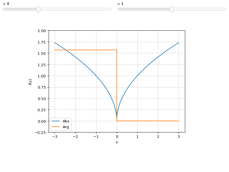
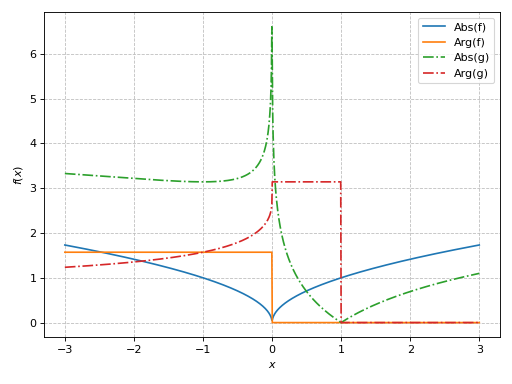
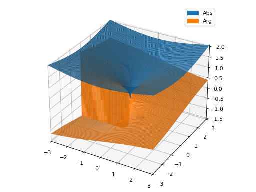
Plot only the absolute value and argument:

>>> graphics(
...     line_abs_arg(sqrt(x), (x, -3, 3), label="f"),
...     line_abs_arg(log(x), (x, -3, 3), label="g",
...         rendering_kw={"linestyle": "-."}),
... )
Plot object containing:
[0]: cartesian line: abs(sqrt(x)) for x over (-3, 3)
[1]: cartesian line: arg(sqrt(x)) for x over (-3, 3)
[2]: cartesian line: abs(log(x)) for x over (-3, 3)
[3]: cartesian line: arg(log(x)) for x over (-3, 3)

(Source code, png)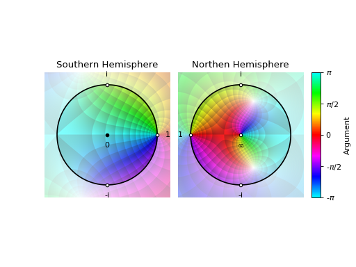

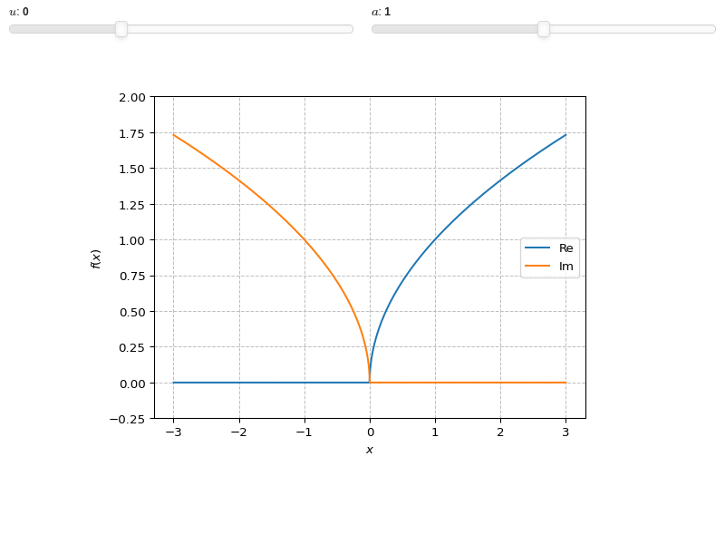
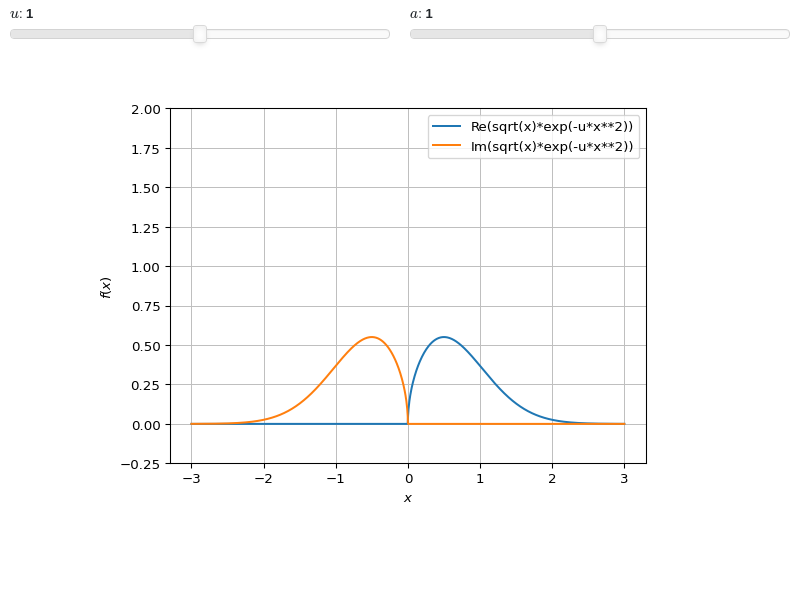
Interactive-widget plot. Refer to the interactive sub-module documentation to learn more about the params dictionary. This plot illustrates:

• the use of prange (parametric plotting range).

• for line_abs_arg, symbols going into prange must be real.

• the use of the params dictionary to specify sliders in their basic form: (default, min, max).

from sympy import *
from spb import *
x, u = symbols("x, u")
a = symbols("a", real=True)
graphics(
    line_abs_arg(
        (sqrt(x) + u) * exp(-u * x**2), prange(x, -3*a, 3*a),
        params={u: (0, -1, 2), a: (1, 0, 2)}),
    ylim=(-0.25, 2))

(Source code, small.png)

spb.graphics.complex_analysis.line_real_imag(expr, range_x=None, label=None, rendering_kw=None, real=True, imag=True, **kwargs)

Plot the real and imaginary part of a complex function f(x) with x in Reals.

Parameters:

expr

It can either be a symbolic expression representing the function of one variable to be plotted, or a numerical function of one variable, supporting vectorization. In the latter case the following keyword arguments are not supported: params, sum_bound.

range_xtuple, Tuple

A 3-tuple (symb, min, max) denoting the range of the x variable. Default values: min=-10 and max=10.

labelstr

Set the label associated to this series, which will be eventually shown on the legend or colorbar.

rendering_kwdict

A dictionary of keyword arguments to be passed to the renderers in order to further customize the appearance of the line. Here are some useful links for the supported plotting libraries:

• Matplotlib:

  • for solid lines: https://matplotlib.org/stable/api/_as_gen/matplotlib.pyplot.plot.html

  • for colormap-based lines: https://matplotlib.org/stable/api/collections_api.html#matplotlib.collections.LineCollection

  • for scatters: https://matplotlib.org/stable/api/_as_gen/matplotlib.pyplot.scatter.html

• Bokeh:

  • for solid lines: https://docs.bokeh.org/en/latest/docs/reference/plotting.html#bokeh.plotting.Figure.line

  • for scatter: https://docs.bokeh.org/en/latest/docs/reference/plotting/figure.html#bokeh.plotting.Figure.scatter

• Plotly: https://plotly.com/python/line-and-scatter/

color_func

A color function to be applied to the numerical data. It can be:

• A numerical function of 2 variables, x, y (the points computed by the internal algorithm) supporting vectorization.

• A symbolic expression having at most as many free symbols as expr.

• None: the default value (no color mapping).

colorbarbool

Toggle the visibility of the colorbar associated to the current data series. Note that a colorbar is only visible if use_cm=True and color_func is not None. Default value: True.

colorbar_ticks_formattertick_formatter_multiples_of

An object of type tick_formatter_multiples_of which will be used to place tick values on the colorbar at each multiple of a specified quantity. This only works when use_cm=True.

detect_polesbool, str

Chose whether to detect and correctly plot the roots of the denominator. There are two algorithms at work:

1. based on the gradient of the numerical data, it introduces NaN values at locations where the steepness is greater than some threshold. This splits the line into multiple segments. To improve detection, increase the number of discretization points n and/or change the value of eps. This algorithm can be used to visualize jump discontinuities as well as essential discontinuities.

2. a symbolic approach based on the continuous_domain function from the sympy.calculus.util module, which computes the locations of essential discontinuities. If any are found, vertical lines will be shown.

Possible options:

• False: No poles detection

• True: Poles detection with the numerical algorithm

• ‘symbolic’: Poles detection with numerical and symbolic algorithms

Default value: False.

epsfloat

An arbitrary small value used by the detect_poles numerical algorithm. Before changing this value, it is recommended to increase the number of discretization points. Related parameters: detect_poles. It must be: 0 ≤ eps < ∞. Default value: 0.01.

excludelist

List of x-coordinates to be excluded from evaluation. In practice, it introduces discontinuities in the resulting line.

force_real_evalbool

By default, numerical evaluation is performed over complex numbers, which is slower but produces correct results. However, when the symbolic expression is converted to a numerical function with lambdify, the resulting function may not like to be evaluated over complex numbers. In such cases, forcing the evaluation to be performed over real numbers might be a good choice. The plotting module should be able to detect such occurences and automatically activate this option. If that is not the case, or evaluation performance is of paramount importance, set this parameter to True, but be aware that it might produce wrong results. Default value: False.

is_filledbool

Whether scatter’s markers are filled or void. Default value: True.

is_scatterbool

If True it represent a scatter plot, otherwise a continuous line. Default value: False.

line_color

For back-compatibility with old sympy.plotting. Use rendering_kw in order to fully customize the appearance of the line/scatter.

modules

Specify the evaluation modules to be used by lambdify. If not specified, the evaluation will be done with NumPy/SciPy.

n1int

Number of discretization points along the parameter to be used in the numerical evaluation. An alias of this parameter is n. Related parameters: xscale. It must be: 2 ≤ n1 < ∞. Default value: 1000.

only_integersbool

Discretize the domain using only integer numbers. When this parameter is True, the number of discretization points is choosen by the algorithm. Default value: False.

paramsdict, optional

A dictionary mapping symbols to parameters. If provided, this dictionary enables the interactive-widgets plot.

When calling a plotting function, the parameter can be specified with:

• a widget from the ipywidgets module.

• a widget from the panel module.

• a tuple of the form:

  (default, min, max, N, tick_format, label, spacing), which will instantiate a ipywidgets.widgets.widget_float.FloatSlider or a ipywidgets.widgets.widget_float.FloatLogSlider, depending on the spacing strategy. In particular:

  • default, min, maxfloat

    Default value, minimum value and maximum value of the slider, respectively. Must be finite numbers. The order of these 3 numbers is not important: the module will figure it out which is what.

  • Nint, optional

    Number of steps of the slider.

  • tick_formatstr or None, optional

    Provide a formatter for the tick value of the slider. Default to ".2f".

  • label: str, optional

    Custom text associated to the slider.

  • spacingstr, optional

    Specify the discretization spacing. Default to "linear", can be changed to "log".

Notes:

1. parameters cannot be linked together (ie, one parameter cannot depend on another one).

2. If a widget returns multiple numerical values (like panel.widgets.slider.RangeSlider or ipywidgets.widgets.widget_float.FloatRangeSlider), then a corresponding number of symbols must be provided.

Here follows a couple of examples. If imodule="panel":

import panel as pn
params = {
    a: (1, 0, 5), # slider from 0 to 5, with default value of 1
    b: pn.widgets.FloatSlider(value=1, start=0, end=5), # same slider as above
    (c, d): pn.widgets.RangeSlider(value=(-1, 1), start=-3, end=3, step=0.1)
}

Or with imodule="ipywidgets":

import ipywidgets as w
params = {
    a: (1, 0, 5), # slider from 0 to 5, with default value of 1
    b: w.FloatSlider(value=1, min=0, max=5), # same slider as above
    (c, d): w.FloatRangeSlider(value=(-1, 1), min=-3, max=3, step=0.1)
}

When instantiating a data series directly, params must be a dictionary mapping symbols to numerical values.

Let series be any data series. Then series.params returns a dictionary mapping symbols to numerical values.

poles_locationslist

When detect_poles="symbolic", stores the location of the computed poles (essential discontinuities) so that they can be appropriately rendered.

poles_rendering_kwdict

Rendering kw used to customize the appearance of vertical lines representing essential discontinuities. Related parameters: poles_locations.

show_in_legendbool

Toggle the visibility of the data series on the legend. Default value: True.

stepsNoneType, bool, str

If set, it connects consecutive points with steps rather than straight segments. Possible options: [‘pre’, ‘post’, ‘mid’, True, False, None] Default value: False.

sum_boundint

When plotting sums, the expression will be pre-processed in order to replace lower/upper bounds set to +/- infinity with this +/- numerical value. Note: the higher this number, the slower the evaluation, but the more accurate the plot. It must be: 0 ≤ sum_bound < ∞. Default value: 1000.

txcallable

Numerical transformation function to be applied to the data on the x-axis.

tycallable

Numerical transformation function to be applied to the data on the y-axis.

unwrapbool, dict

Whether to use numpy.unwrap() on the computed coordinates in order to get rid of discontinuities. It can be:

• False: do not use np.unwrap().

• True: use np.unwrap() with default keyword arguments.

• dictionary of keyword arguments passed to np.unwrap().

use_cmbool

Toggle the use of a colormap. By default, some series might use a colormap to display the necessary data. Setting this attribute to False will inform the associated renderer to use solid color. Related parameters: color_func. Default value: False.

xscalestr

Discretization strategy along the x-direction. Related parameters: n1. Possible options: [‘linear’, ‘log’] Default value: ‘linear’.

Returns:

serieslist

A list containing instances of LineOver1DRangeSeries.

See also

spb.graphics.functions_2d.line, line_abs_arg, line_abs_arg_colored

Notes

Given a symbolic expression, there are two possible way to create a real/imag plot:

1. Apply Sympy’s re or im to the symbolic expression, then evaluates it.

2. Evaluates the symbolic expression over the provided range in order to get complex values, then extract the real/imaginary parts with Numpy.

For performance reasons, line_real_imag implements the second approach. In fact, SymPy’s re and im functions evaluate their arguments, potentially creating unecessarely long symbolic expressions that requires a lot of time lambdified and evaluated.

Another thing to be aware of is branch cuts of complex-valued functions. The plotting module attempt to evaluate a symbolic expression using complex numbers. Depending on the evaluation module being used, we might get different results. For example, the following two expressions are equal when x > 0:

>>> from sympy import symbols, im, Rational
>>> from spb import *
>>> x = symbols('x', positive=True)
>>> x_generic = symbols("x")
>>> e1 = (1 / x)**(Rational(6, 5))
>>> e2 = x**(-Rational(6, 5))
>>> e2.equals(e1)
True
>>> e3 = (1 / x_generic)**(Rational(6, 5))
>>> e4 = x_generic**(-Rational(6, 5))
>>> e4.equals(e3) is None
True
>>> graphics(
...     line_real_imag(e3, label="e3", real=False,
...         detect_poles="symbolic"),
...     line_real_imag(e4, label="e4", real=False,
...         detect_poles="symbolic"),
...     ylim=(-5, 5))
Plot object containing:
[0]: cartesian line: im((1/x)**(6/5)) for x over (-10, 10)
[1]: cartesian line: im(x**(-6/5)) for x over (-10, 10)

(Source code, png)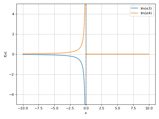

The result computed by the plotting module might feels off: the two expressions are different, but according to the plot they are the same. Someone could say that the imaginary part of e3 or e4 should be negative when x < 0. We can evaluate the expressions with mpmath:

>>> graphics(
...     line_real_imag(e3, label="e3", real=False,
...         detect_poles="symbolic", modules="mpmath"),
...     line_real_imag(e4, label="e4", real=False,
...         detect_poles="symbolic", modules="mpmath"),
...     ylim=(-5, 5))
Plot object containing:
[0]: cartesian line: im((1/x)**(6/5)) for x over (-10, 10)
[1]: cartesian line: im(x**(-6/5)) for x over (-10, 10)

(Source code, png)

With mpmath we see that e3 and e4 are indeed different.

Examples

>>> from sympy import symbols, sqrt, log
>>> from spb import *
>>> x = symbols('x')

(Source code)

Plot only the absolute value and argument:

>>> graphics(
...     line_real_imag(sqrt(x), (x, -3, 3), label="f"))
Plot object containing:
[0]: cartesian line: re(sqrt(x)) for x over (-3, 3)
[1]: cartesian line: im(sqrt(x)) for x over (-3, 3)

(Source code, png)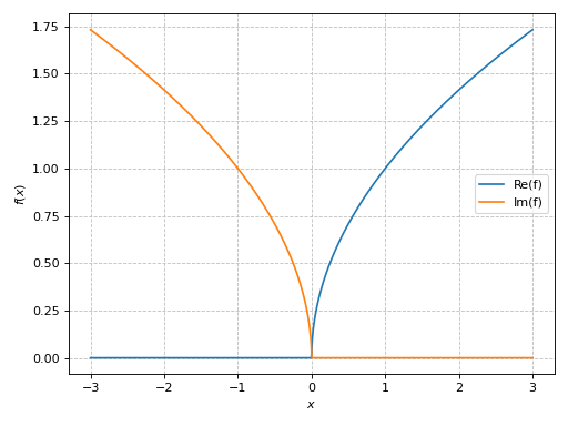

Interactive-widget plot. Refer to the interactive sub-module documentation to learn more about the params dictionary. This plot illustrates:

• the use of prange (parametric plotting range).

• for line_real_imag, symbols going into prange must be real.

• the use of the params dictionary to specify sliders in their basic form: (default, min, max).

from sympy import *
from spb import *
x, u = symbols("x, u")
a = symbols("a", real=True)
graphics(
    line_real_imag((sqrt(x) + u) * exp(-u * x**2), prange(x, -3*a, 3*a),
        params={u: (0, -1, 2), a: (1, 0, 2)}),
    ylim=(-0.25, 2))

(Source code, small.png)

spb.graphics.complex_analysis.surface_abs_arg(expr, range_c=None, label=None, rendering_kw=None, abs=True, arg=True, **kwargs)

Plot the absolute value and/or the argument of a complex function f(x) with x in Complex.

Parameters:

expr

The expression representing the complex function to be plotted.

range_ctuple, Tuple

A 3-tuple (symb, min, max) denoting the range of the complex variable. Default values: min=-10-10j and max=10+10j.

labelstr

Set the label associated to this series, which will be eventually shown on the legend or colorbar.

rendering_kwdict

A dictionary of keyword arguments to be passed to the renderers in order to further customize the appearance of the surface. Here are some useful links for the supported plotting libraries:

• Matplotlib: https://matplotlib.org/stable/api/_as_gen/mpl_toolkits.mplot3d.axes3d.Axes3D.html#mpl_toolkits.mplot3d.axes3d.Axes3D.plot_surface

• Plotly: https://plotly.com/python/3d-surface-plots/

• K3D-Jupyter: look at the documentation of k3d.mesh.

absboolean, optional

Show/hide the absolute value. Default to True (visible).

argboolean, optional

Show/hide the argument. Default to True (visible).

color_func

Define a custom color mapping to be used when use_cm=True. It can either be:

• A numerical function supporting vectorization. The arity can be:

  • 2 arguments: f(x, y) where x, y are the coordinates of the points.

  • 3 arguments: f(x, y, z) where x, y, z are the coordinates of the points.

• A symbolic expression having at most as many free symbols as expr.

• None: the default value (color mapping according to the z coordinate).

colorbarbool

Toggle the visibility of the colorbar associated to the current data series. Note that a colorbar is only visible if use_cm=True and color_func is not None. Default value: True.

colorbar_ticks_formattertick_formatter_multiples_of

An object of type tick_formatter_multiples_of which will be used to place tick values on the colorbar at each multiple of a specified quantity. This only works when use_cm=True.

force_real_evalbool

By default, numerical evaluation is performed over complex numbers, which is slower but produces correct results. However, when the symbolic expression is converted to a numerical function with lambdify, the resulting function may not like to be evaluated over complex numbers. In such cases, forcing the evaluation to be performed over real numbers might be a good choice. The plotting module should be able to detect such occurences and automatically activate this option. If that is not the case, or evaluation performance is of paramount importance, set this parameter to True, but be aware that it might produce wrong results. Default value: False.

is_filledbool

If True, used filled contours. Otherwise, use line contours. Relatated parameters: show_clabels. Default value: True.

modules

Specify the evaluation modules to be used by lambdify. If not specified, the evaluation will be done with NumPy/SciPy.

n1int

Number of discretization points along the x-axis (real part) to be used in the evaluation. Related parameters: xscale. It must be: 2 ≤ n1 < ∞. Default value: 300.

n2int

Number of discretization points along the y-axis (imaginary part) to be used in the evaluation. Related parameters: yscale. It must be: 2 ≤ n2 < ∞. Default value: 300.

only_integersbool

Discretize the domain using only integer numbers. When this parameter is True, the number of discretization points is choosen by the algorithm. Default value: False.

paramsdict, optional

A dictionary mapping symbols to parameters. If provided, this dictionary enables the interactive-widgets plot.

When calling a plotting function, the parameter can be specified with:

• a widget from the ipywidgets module.

• a widget from the panel module.

• a tuple of the form:

  (default, min, max, N, tick_format, label, spacing), which will instantiate a ipywidgets.widgets.widget_float.FloatSlider or a ipywidgets.widgets.widget_float.FloatLogSlider, depending on the spacing strategy. In particular:

  • default, min, maxfloat

    Default value, minimum value and maximum value of the slider, respectively. Must be finite numbers. The order of these 3 numbers is not important: the module will figure it out which is what.

  • Nint, optional

    Number of steps of the slider.

  • tick_formatstr or None, optional

    Provide a formatter for the tick value of the slider. Default to ".2f".

  • label: str, optional

    Custom text associated to the slider.

  • spacingstr, optional

    Specify the discretization spacing. Default to "linear", can be changed to "log".

Notes:

1. parameters cannot be linked together (ie, one parameter cannot depend on another one).

2. If a widget returns multiple numerical values (like panel.widgets.slider.RangeSlider or ipywidgets.widgets.widget_float.FloatRangeSlider), then a corresponding number of symbols must be provided.

Here follows a couple of examples. If imodule="panel":

import panel as pn
params = {
    a: (1, 0, 5), # slider from 0 to 5, with default value of 1
    b: pn.widgets.FloatSlider(value=1, start=0, end=5), # same slider as above
    (c, d): pn.widgets.RangeSlider(value=(-1, 1), start=-3, end=3, step=0.1)
}

Or with imodule="ipywidgets":

import ipywidgets as w
params = {
    a: (1, 0, 5), # slider from 0 to 5, with default value of 1
    b: w.FloatSlider(value=1, min=0, max=5), # same slider as above
    (c, d): w.FloatRangeSlider(value=(-1, 1), min=-3, max=3, step=0.1)
}

When instantiating a data series directly, params must be a dictionary mapping symbols to numerical values.

Let series be any data series. Then series.params returns a dictionary mapping symbols to numerical values.

show_clabelsbool

Toggle the label’s visibility of contour lines. It only works when is_filled=False. Note that some backend might not implement this feature. Relatated parameters: is_filled. Default value: True.

show_in_legendbool

Toggle the visibility of the data series on the legend. Default value: True.

sum_boundint

When plotting sums, the expression will be pre-processed in order to replace lower/upper bounds set to +/- infinity with this +/- numerical value. Note: the higher this number, the slower the evaluation, but the more accurate the plot. It must be: 0 ≤ sum_bound < ∞. Default value: 1000.

surface_color

For back-compatibility with old sympy.plotting. Use rendering_kw in order to fully customize the appearance of the surface.

txcallable

Numerical transformation function to be applied to the data on the x-axis.

tycallable

Numerical transformation function to be applied to the data on the y-axis.

tzcallable

Numerical transformation function to be applied to the data on the z-axis.

use_cmbool

Toggle the use of a colormap. By default, some series might use a colormap to display the necessary data. Setting this attribute to False will inform the associated renderer to use solid color. Related parameters: color_func. Default value: False.

xscalestr

Discretization strategy along the x-direction (real part). Related parameters: n1. Possible options: [‘linear’, ‘log’] Default value: ‘linear’.

yscalestr

Discretization strategy along the y-direction (imaginary part). Related parameters: n12. Possible options: [‘linear’, ‘log’] Default value: ‘linear’.

Returns:

serieslist

A list containing up two to instance of ComplexSurfaceSeries and possibly multiple instances of Parametric3DLineSeries, if wireframe=True.

See also

spb.graphics.functions_3d.surface, contour_abs_arg, surface_real_imag

contour_abs_arg

Examples

>>> from sympy import symbols, sqrt
>>> from spb import *
>>> x = symbols('x')

(Source code)

>>> graphics(
...     surface_abs_arg(sqrt(x), (x, -3-3j, 3+3j), n=101))
Plot object containing:
[0]: complex cartesian surface: abs(sqrt(x)) for re(x) over (-3.0, 3.0) and im(x) over (-3.0, 3.0)
[1]: complex cartesian surface: arg(sqrt(x)) for re(x) over (-3.0, 3.0) and im(x) over (-3.0, 3.0)

(Source code, png)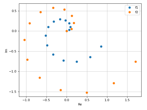

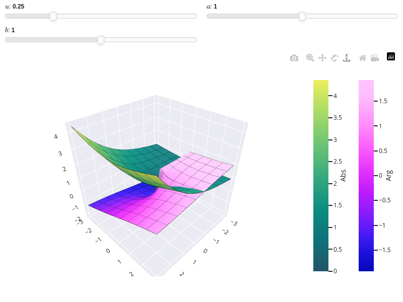
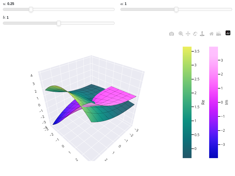
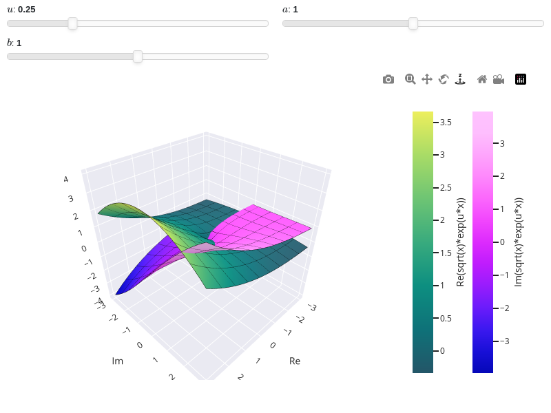
Interactive-widget plot. Refer to the interactive sub-module documentation to learn more about the params dictionary. This plot illustrates:

• the use of prange (parametric plotting range).

• the use of the params dictionary to specify sliders in their basic form: (default, min, max).

from sympy import *
from spb import *
x, u, a, b = symbols("x, u, a, b")
graphics(
    surface_abs_arg(
        sqrt(x) * exp(u * x), prange(x, -3*a-b*3j, 3*a+b*3j),
        n=25, wireframe=True, wf_rendering_kw={"line_width": 1},
        use_cm=True, params={
            u: (0.25, 0, 1),
            a: (1, 0, 2),
            b: (1, 0, 2)
        }),
        backend=PB, aspect="cube")

(Source code, small.png)

spb.graphics.complex_analysis.contour_abs_arg(expr, range_c=None, label=None, rendering_kw=None, abs=True, arg=True, **kwargs)

Plot contours of the absolute value and/or the argument of a complex function f(x) with x in Complex.

Parameters:

expr

The expression representing the complex function to be plotted.

range_ctuple, Tuple

A 3-tuple (symb, min, max) denoting the range of the complex variable. Default values: min=-10-10j and max=10+10j.

labelstr

Set the label associated to this series, which will be eventually shown on the legend or colorbar.

rendering_kwdict

A dictionary of keyword arguments to be passed to the renderers in order to further customize the appearance of the surface. Here are some useful links for the supported plotting libraries:

• Matplotlib: https://matplotlib.org/stable/api/_as_gen/mpl_toolkits.mplot3d.axes3d.Axes3D.html#mpl_toolkits.mplot3d.axes3d.Axes3D.plot_surface

• Plotly: https://plotly.com/python/3d-surface-plots/

• K3D-Jupyter: look at the documentation of k3d.mesh.

absboolean, optional

Show/hide the absolute value. Default to True (visible).

argboolean, optional

Show/hide the argument. Default to True (visible).

color_func

Define a custom color mapping to be used when use_cm=True. It can either be:

• A numerical function supporting vectorization. The arity can be:

  • 2 arguments: f(x, y) where x, y are the coordinates of the points.

  • 3 arguments: f(x, y, z) where x, y, z are the coordinates of the points.

• A symbolic expression having at most as many free symbols as expr.

• None: the default value (color mapping according to the z coordinate).

colorbarbool

Toggle the visibility of the colorbar associated to the current data series. Note that a colorbar is only visible if use_cm=True and color_func is not None. Default value: True.

colorbar_ticks_formattertick_formatter_multiples_of

An object of type tick_formatter_multiples_of which will be used to place tick values on the colorbar at each multiple of a specified quantity. This only works when use_cm=True.

force_real_evalbool

By default, numerical evaluation is performed over complex numbers, which is slower but produces correct results. However, when the symbolic expression is converted to a numerical function with lambdify, the resulting function may not like to be evaluated over complex numbers. In such cases, forcing the evaluation to be performed over real numbers might be a good choice. The plotting module should be able to detect such occurences and automatically activate this option. If that is not the case, or evaluation performance is of paramount importance, set this parameter to True, but be aware that it might produce wrong results. Default value: False.

is_filledbool

If True, used filled contours. Otherwise, use line contours. Relatated parameters: show_clabels. Default value: True.

modules

Specify the evaluation modules to be used by lambdify. If not specified, the evaluation will be done with NumPy/SciPy.

n1int

Number of discretization points along the x-axis (real part) to be used in the evaluation. Related parameters: xscale. It must be: 2 ≤ n1 < ∞. Default value: 300.

n2int

Number of discretization points along the y-axis (imaginary part) to be used in the evaluation. Related parameters: yscale. It must be: 2 ≤ n2 < ∞. Default value: 300.

only_integersbool

Discretize the domain using only integer numbers. When this parameter is True, the number of discretization points is choosen by the algorithm. Default value: False.

paramsdict, optional

A dictionary mapping symbols to parameters. If provided, this dictionary enables the interactive-widgets plot.

When calling a plotting function, the parameter can be specified with:

• a widget from the ipywidgets module.

• a widget from the panel module.

• a tuple of the form:

  (default, min, max, N, tick_format, label, spacing), which will instantiate a ipywidgets.widgets.widget_float.FloatSlider or a ipywidgets.widgets.widget_float.FloatLogSlider, depending on the spacing strategy. In particular:

  • default, min, maxfloat

    Default value, minimum value and maximum value of the slider, respectively. Must be finite numbers. The order of these 3 numbers is not important: the module will figure it out which is what.

  • Nint, optional

    Number of steps of the slider.

  • tick_formatstr or None, optional

    Provide a formatter for the tick value of the slider. Default to ".2f".

  • label: str, optional

    Custom text associated to the slider.

  • spacingstr, optional

    Specify the discretization spacing. Default to "linear", can be changed to "log".

Notes:

1. parameters cannot be linked together (ie, one parameter cannot depend on another one).

2. If a widget returns multiple numerical values (like panel.widgets.slider.RangeSlider or ipywidgets.widgets.widget_float.FloatRangeSlider), then a corresponding number of symbols must be provided.

Here follows a couple of examples. If imodule="panel":

import panel as pn
params = {
    a: (1, 0, 5), # slider from 0 to 5, with default value of 1
    b: pn.widgets.FloatSlider(value=1, start=0, end=5), # same slider as above
    (c, d): pn.widgets.RangeSlider(value=(-1, 1), start=-3, end=3, step=0.1)
}

Or with imodule="ipywidgets":

import ipywidgets as w
params = {
    a: (1, 0, 5), # slider from 0 to 5, with default value of 1
    b: w.FloatSlider(value=1, min=0, max=5), # same slider as above
    (c, d): w.FloatRangeSlider(value=(-1, 1), min=-3, max=3, step=0.1)
}

When instantiating a data series directly, params must be a dictionary mapping symbols to numerical values.

Let series be any data series. Then series.params returns a dictionary mapping symbols to numerical values.

show_clabelsbool

Toggle the label’s visibility of contour lines. It only works when is_filled=False. Note that some backend might not implement this feature. Relatated parameters: is_filled. Default value: True.

show_in_legendbool

Toggle the visibility of the data series on the legend. Default value: True.

sum_boundint

When plotting sums, the expression will be pre-processed in order to replace lower/upper bounds set to +/- infinity with this +/- numerical value. Note: the higher this number, the slower the evaluation, but the more accurate the plot. It must be: 0 ≤ sum_bound < ∞. Default value: 1000.

surface_color

For back-compatibility with old sympy.plotting. Use rendering_kw in order to fully customize the appearance of the surface.

txcallable

Numerical transformation function to be applied to the data on the x-axis.

tycallable

Numerical transformation function to be applied to the data on the y-axis.

tzcallable

Numerical transformation function to be applied to the data on the z-axis.

use_cmbool

Toggle the use of a colormap. By default, some series might use a colormap to display the necessary data. Setting this attribute to False will inform the associated renderer to use solid color. Related parameters: color_func. Default value: False.

xscalestr

Discretization strategy along the x-direction (real part). Related parameters: n1. Possible options: [‘linear’, ‘log’] Default value: ‘linear’.

yscalestr

Discretization strategy along the y-direction (imaginary part). Related parameters: n12. Possible options: [‘linear’, ‘log’] Default value: ‘linear’.

Returns:

serieslist

A list containing up two to instance of ComplexSurfaceSeries.

See also

spb.graphics.functions_2d.contour, contour_real_imag, surface_real_imag

surface_abs_arg

Examples

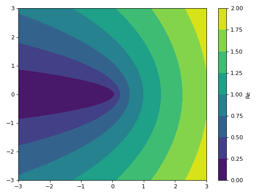
>>> from sympy import symbols, sqrt
>>> from spb import *
>>> x = symbols('x')

(Source code)

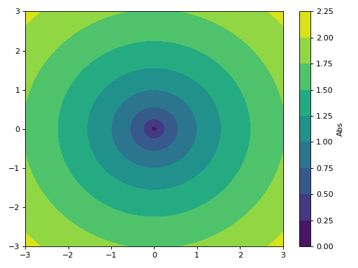
>>> graphics(
...     contour_abs_arg(sqrt(x), (x, -3-3j, 3+3j), arg=False),
...     grid=False)
Plot object containing:
[0]: complex contour: abs(sqrt(x)) for re(x) over (-3.0, 3.0) and im(x) over (-3.0, 3.0)

(Source code, png)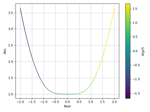

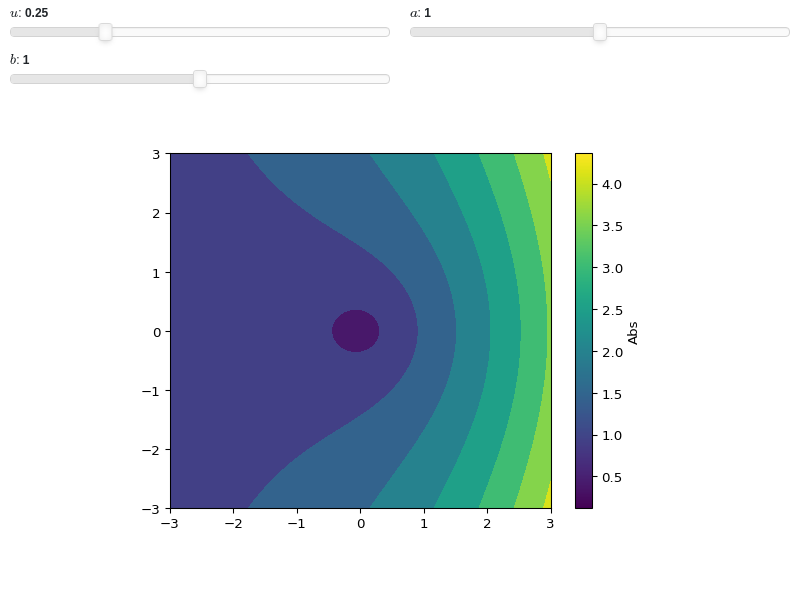
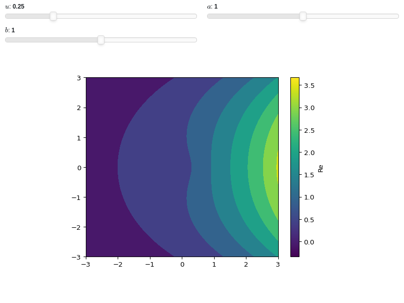
Interactive-widget plot. Refer to the interactive sub-module documentation to learn more about the params dictionary. This plot illustrates:

• the use of prange (parametric plotting range).

• the use of the params dictionary to specify sliders in their basic form: (default, min, max).

from sympy import *
from spb import *
x, u, a, b = symbols("x, u, a, b")
graphics(
    contour_abs_arg(
        sqrt(x) * exp(u * x), prange(x, -3*a-b*3j, 3*a+b*3j),
        arg=False, use_cm=True,
        params={
            u: (0.25, 0, 1),
            a: (1, 0, 2),
            b: (1, 0, 2)
        }),
    grid=False)

(Source code, small.png)

spb.graphics.complex_analysis.surface_real_imag(expr, range_c=None, label=None, rendering_kw=None, real=True, imag=True, **kwargs)

Plot the real and imaginary part of a complex function f(x) with x in Complex.

Parameters:

expr

The expression representing the complex function to be plotted.

range_ctuple, Tuple

A 3-tuple (symb, min, max) denoting the range of the complex variable. Default values: min=-10-10j and max=10+10j.

labelstr

Set the label associated to this series, which will be eventually shown on the legend or colorbar.

rendering_kwdict

A dictionary of keyword arguments to be passed to the renderers in order to further customize the appearance of the surface. Here are some useful links for the supported plotting libraries:

• Matplotlib: https://matplotlib.org/stable/api/_as_gen/mpl_toolkits.mplot3d.axes3d.Axes3D.html#mpl_toolkits.mplot3d.axes3d.Axes3D.plot_surface

• Plotly: https://plotly.com/python/3d-surface-plots/

• K3D-Jupyter: look at the documentation of k3d.mesh.

realboolean, optional

Show/hide the real part. Default to True (visible).

imagboolean, optional

Show/hide the imaginary part. Default to True (visible).

color_func

Define a custom color mapping to be used when use_cm=True. It can either be:

• A numerical function supporting vectorization. The arity can be:

  • 2 arguments: f(x, y) where x, y are the coordinates of the points.

  • 3 arguments: f(x, y, z) where x, y, z are the coordinates of the points.

• A symbolic expression having at most as many free symbols as expr.

• None: the default value (color mapping according to the z coordinate).

colorbarbool

Toggle the visibility of the colorbar associated to the current data series. Note that a colorbar is only visible if use_cm=True and color_func is not None. Default value: True.

colorbar_ticks_formattertick_formatter_multiples_of

An object of type tick_formatter_multiples_of which will be used to place tick values on the colorbar at each multiple of a specified quantity. This only works when use_cm=True.

force_real_evalbool

By default, numerical evaluation is performed over complex numbers, which is slower but produces correct results. However, when the symbolic expression is converted to a numerical function with lambdify, the resulting function may not like to be evaluated over complex numbers. In such cases, forcing the evaluation to be performed over real numbers might be a good choice. The plotting module should be able to detect such occurences and automatically activate this option. If that is not the case, or evaluation performance is of paramount importance, set this parameter to True, but be aware that it might produce wrong results. Default value: False.

is_filledbool

If True, used filled contours. Otherwise, use line contours. Relatated parameters: show_clabels. Default value: True.

modules

Specify the evaluation modules to be used by lambdify. If not specified, the evaluation will be done with NumPy/SciPy.

n1int

Number of discretization points along the x-axis (real part) to be used in the evaluation. Related parameters: xscale. It must be: 2 ≤ n1 < ∞. Default value: 300.

n2int

Number of discretization points along the y-axis (imaginary part) to be used in the evaluation. Related parameters: yscale. It must be: 2 ≤ n2 < ∞. Default value: 300.

only_integersbool

Discretize the domain using only integer numbers. When this parameter is True, the number of discretization points is choosen by the algorithm. Default value: False.

paramsdict, optional

A dictionary mapping symbols to parameters. If provided, this dictionary enables the interactive-widgets plot.

When calling a plotting function, the parameter can be specified with:

• a widget from the ipywidgets module.

• a widget from the panel module.

• a tuple of the form:

  (default, min, max, N, tick_format, label, spacing), which will instantiate a ipywidgets.widgets.widget_float.FloatSlider or a ipywidgets.widgets.widget_float.FloatLogSlider, depending on the spacing strategy. In particular:

  • default, min, maxfloat

    Default value, minimum value and maximum value of the slider, respectively. Must be finite numbers. The order of these 3 numbers is not important: the module will figure it out which is what.

  • Nint, optional

    Number of steps of the slider.

  • tick_formatstr or None, optional

    Provide a formatter for the tick value of the slider. Default to ".2f".

  • label: str, optional

    Custom text associated to the slider.

  • spacingstr, optional

    Specify the discretization spacing. Default to "linear", can be changed to "log".

Notes:

1. parameters cannot be linked together (ie, one parameter cannot depend on another one).

2. If a widget returns multiple numerical values (like panel.widgets.slider.RangeSlider or ipywidgets.widgets.widget_float.FloatRangeSlider), then a corresponding number of symbols must be provided.

Here follows a couple of examples. If imodule="panel":

import panel as pn
params = {
    a: (1, 0, 5), # slider from 0 to 5, with default value of 1
    b: pn.widgets.FloatSlider(value=1, start=0, end=5), # same slider as above
    (c, d): pn.widgets.RangeSlider(value=(-1, 1), start=-3, end=3, step=0.1)
}

Or with imodule="ipywidgets":

import ipywidgets as w
params = {
    a: (1, 0, 5), # slider from 0 to 5, with default value of 1
    b: w.FloatSlider(value=1, min=0, max=5), # same slider as above
    (c, d): w.FloatRangeSlider(value=(-1, 1), min=-3, max=3, step=0.1)
}

When instantiating a data series directly, params must be a dictionary mapping symbols to numerical values.

Let series be any data series. Then series.params returns a dictionary mapping symbols to numerical values.

show_clabelsbool

Toggle the label’s visibility of contour lines. It only works when is_filled=False. Note that some backend might not implement this feature. Relatated parameters: is_filled. Default value: True.

show_in_legendbool

Toggle the visibility of the data series on the legend. Default value: True.

sum_boundint

When plotting sums, the expression will be pre-processed in order to replace lower/upper bounds set to +/- infinity with this +/- numerical value. Note: the higher this number, the slower the evaluation, but the more accurate the plot. It must be: 0 ≤ sum_bound < ∞. Default value: 1000.

surface_color

For back-compatibility with old sympy.plotting. Use rendering_kw in order to fully customize the appearance of the surface.

txcallable

Numerical transformation function to be applied to the data on the x-axis.

tycallable

Numerical transformation function to be applied to the data on the y-axis.

tzcallable

Numerical transformation function to be applied to the data on the z-axis.

use_cmbool

Toggle the use of a colormap. By default, some series might use a colormap to display the necessary data. Setting this attribute to False will inform the associated renderer to use solid color. Related parameters: color_func. Default value: False.

xscalestr

Discretization strategy along the x-direction (real part). Related parameters: n1. Possible options: [‘linear’, ‘log’] Default value: ‘linear’.

yscalestr

Discretization strategy along the y-direction (imaginary part). Related parameters: n12. Possible options: [‘linear’, ‘log’] Default value: ‘linear’.

Returns:

serieslist

A list containing up two to instance of ComplexSurfaceSeries and possibly multiple instances of Parametric3DLineSeries, if wireframe=True.

See also

spb.graphics.functions_3d.surface, contour_abs_arg, contour_real_imag

surface_abs_arg

Examples

>>> from sympy import symbols, sqrt
>>> from spb import *
>>> x = symbols('x')

(Source code)

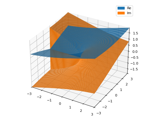
>>> graphics(
...     surface_real_imag(sqrt(x), (x, -3-3j, 3+3j), n=101))
Plot object containing:
[0]: complex cartesian surface: re(sqrt(x)) for re(x) over (-3.0, 3.0) and im(x) over (-3.0, 3.0)
[1]: complex cartesian surface: im(sqrt(x)) for re(x) over (-3.0, 3.0) and im(x) over (-3.0, 3.0)

(Source code, png)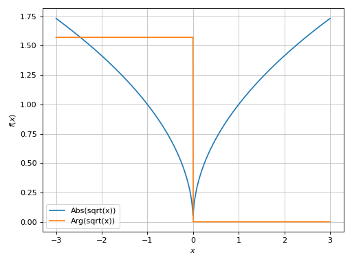

Interactive-widget plot. Refer to the interactive sub-module documentation to learn more about the params dictionary. This plot illustrates:

• the use of prange (parametric plotting range).

• the use of the params dictionary to specify sliders in their basic form: (default, min, max).

from sympy import *
from spb import *
x, u, a, b = symbols("x, u, a, b")
graphics(
    surface_real_imag(
        sqrt(x) * exp(u * x), prange(x, -3*a-b*3j, 3*a+b*3j),
        n=25, wireframe=True, wf_rendering_kw={"line_width": 1},
        use_cm=True, params={
            u: (0.25, 0, 1),
            a: (1, 0, 2),
            b: (1, 0, 2)
        }),
        backend=PB, aspect="cube")

(Source code, small.png)

spb.graphics.complex_analysis.contour_real_imag(expr, range_c=None, label=None, rendering_kw=None, real=True, imag=True, **kwargs)

Plot contours of the real and imaginary parts of a complex function f(x) with x in Complex.

Parameters:

expr

The expression representing the complex function to be plotted.

range_ctuple, Tuple

A 3-tuple (symb, min, max) denoting the range of the complex variable. Default values: min=-10-10j and max=10+10j.

labelstr

Set the label associated to this series, which will be eventually shown on the legend or colorbar.

rendering_kwdict

A dictionary of keyword arguments to be passed to the renderers in order to further customize the appearance of the surface. Here are some useful links for the supported plotting libraries:

• Matplotlib: https://matplotlib.org/stable/api/_as_gen/mpl_toolkits.mplot3d.axes3d.Axes3D.html#mpl_toolkits.mplot3d.axes3d.Axes3D.plot_surface

• Plotly: https://plotly.com/python/3d-surface-plots/

• K3D-Jupyter: look at the documentation of k3d.mesh.

realboolean, optional

Show/hide the real part. Default to True (visible).

imagboolean, optional

Show/hide the imaginary part. Default to True (visible).

color_func

Define a custom color mapping to be used when use_cm=True. It can either be:

• A numerical function supporting vectorization. The arity can be:

  • 2 arguments: f(x, y) where x, y are the coordinates of the points.

  • 3 arguments: f(x, y, z) where x, y, z are the coordinates of the points.

• A symbolic expression having at most as many free symbols as expr.

• None: the default value (color mapping according to the z coordinate).

colorbarbool

Toggle the visibility of the colorbar associated to the current data series. Note that a colorbar is only visible if use_cm=True and color_func is not None. Default value: True.

colorbar_ticks_formattertick_formatter_multiples_of

An object of type tick_formatter_multiples_of which will be used to place tick values on the colorbar at each multiple of a specified quantity. This only works when use_cm=True.

force_real_evalbool

By default, numerical evaluation is performed over complex numbers, which is slower but produces correct results. However, when the symbolic expression is converted to a numerical function with lambdify, the resulting function may not like to be evaluated over complex numbers. In such cases, forcing the evaluation to be performed over real numbers might be a good choice. The plotting module should be able to detect such occurences and automatically activate this option. If that is not the case, or evaluation performance is of paramount importance, set this parameter to True, but be aware that it might produce wrong results. Default value: False.

is_filledbool

If True, used filled contours. Otherwise, use line contours. Relatated parameters: show_clabels. Default value: True.

modules

Specify the evaluation modules to be used by lambdify. If not specified, the evaluation will be done with NumPy/SciPy.

n1int

Number of discretization points along the x-axis (real part) to be used in the evaluation. Related parameters: xscale. It must be: 2 ≤ n1 < ∞. Default value: 300.

n2int

Number of discretization points along the y-axis (imaginary part) to be used in the evaluation. Related parameters: yscale. It must be: 2 ≤ n2 < ∞. Default value: 300.

only_integersbool

Discretize the domain using only integer numbers. When this parameter is True, the number of discretization points is choosen by the algorithm. Default value: False.

paramsdict, optional

A dictionary mapping symbols to parameters. If provided, this dictionary enables the interactive-widgets plot.

When calling a plotting function, the parameter can be specified with:

• a widget from the ipywidgets module.

• a widget from the panel module.

• a tuple of the form:

  (default, min, max, N, tick_format, label, spacing), which will instantiate a ipywidgets.widgets.widget_float.FloatSlider or a ipywidgets.widgets.widget_float.FloatLogSlider, depending on the spacing strategy. In particular:

  • default, min, maxfloat

    Default value, minimum value and maximum value of the slider, respectively. Must be finite numbers. The order of these 3 numbers is not important: the module will figure it out which is what.

  • Nint, optional

    Number of steps of the slider.

  • tick_formatstr or None, optional

    Provide a formatter for the tick value of the slider. Default to ".2f".

  • label: str, optional

    Custom text associated to the slider.

  • spacingstr, optional

    Specify the discretization spacing. Default to "linear", can be changed to "log".

Notes:

1. parameters cannot be linked together (ie, one parameter cannot depend on another one).

2. If a widget returns multiple numerical values (like panel.widgets.slider.RangeSlider or ipywidgets.widgets.widget_float.FloatRangeSlider), then a corresponding number of symbols must be provided.

Here follows a couple of examples. If imodule="panel":

import panel as pn
params = {
    a: (1, 0, 5), # slider from 0 to 5, with default value of 1
    b: pn.widgets.FloatSlider(value=1, start=0, end=5), # same slider as above
    (c, d): pn.widgets.RangeSlider(value=(-1, 1), start=-3, end=3, step=0.1)
}

Or with imodule="ipywidgets":

import ipywidgets as w
params = {
    a: (1, 0, 5), # slider from 0 to 5, with default value of 1
    b: w.FloatSlider(value=1, min=0, max=5), # same slider as above
    (c, d): w.FloatRangeSlider(value=(-1, 1), min=-3, max=3, step=0.1)
}

When instantiating a data series directly, params must be a dictionary mapping symbols to numerical values.

Let series be any data series. Then series.params returns a dictionary mapping symbols to numerical values.

show_clabelsbool

Toggle the label’s visibility of contour lines. It only works when is_filled=False. Note that some backend might not implement this feature. Relatated parameters: is_filled. Default value: True.

show_in_legendbool

Toggle the visibility of the data series on the legend. Default value: True.

sum_boundint

When plotting sums, the expression will be pre-processed in order to replace lower/upper bounds set to +/- infinity with this +/- numerical value. Note: the higher this number, the slower the evaluation, but the more accurate the plot. It must be: 0 ≤ sum_bound < ∞. Default value: 1000.

surface_color

For back-compatibility with old sympy.plotting. Use rendering_kw in order to fully customize the appearance of the surface.

txcallable

Numerical transformation function to be applied to the data on the x-axis.

tycallable

Numerical transformation function to be applied to the data on the y-axis.

tzcallable

Numerical transformation function to be applied to the data on the z-axis.

use_cmbool

Toggle the use of a colormap. By default, some series might use a colormap to display the necessary data. Setting this attribute to False will inform the associated renderer to use solid color. Related parameters: color_func. Default value: False.

xscalestr

Discretization strategy along the x-direction (real part). Related parameters: n1. Possible options: [‘linear’, ‘log’] Default value: ‘linear’.

yscalestr

Discretization strategy along the y-direction (imaginary part). Related parameters: n12. Possible options: [‘linear’, ‘log’] Default value: ‘linear’.

Returns:

serieslist

A list containing up two to instance of ComplexSurfaceSeries.

See also

spb.graphics.functions_2d.contour, contour_abs_arg, surface_real_imag

surface_abs_arg

Examples

>>> from sympy import symbols, sqrt
>>> from spb import *
>>> x = symbols('x')

(Source code)

>>> graphics(
...     contour_real_imag(sqrt(x), (x, -3-3j, 3+3j), imag=False),
...     grid=False)
Plot object containing:
[0]: complex contour: re(sqrt(x)) for re(x) over (-3.0, 3.0) and im(x) over (-3.0, 3.0)

(Source code, png)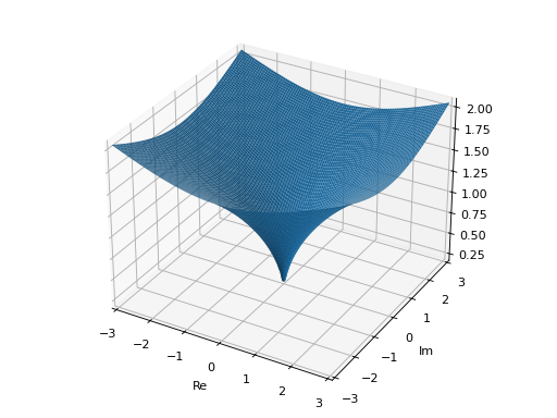

Interactive-widget plot. Refer to the interactive sub-module documentation to learn more about the params dictionary. This plot illustrates:

• the use of prange (parametric plotting range).

• the use of the params dictionary to specify sliders in their basic form: (default, min, max).

from sympy import *
from spb import *
x, u, a, b = symbols("x, u, a, b")
graphics(
    contour_real_imag(
        sqrt(x) * exp(u * x), prange(x, -3*a-b*3j, 3*a+b*3j),
        imag=False, use_cm=True,
        params={
            u: (0.25, 0, 1),
            a: (1, 0, 2),
            b: (1, 0, 2)
        }),
    grid=False)

(Source code, small.png)

spb.graphics.complex_analysis.domain_coloring(expr, range_c=None, label=None, rendering_kw=None, coloring=None, cmap=None, phaseres=20, phaseoffset=0, blevel=0.75, riemann_mask=False, colorbar=True, **kwargs)

Plot an image of the absolute value of a complex function f(x) colored by its argument, with x in Complex.

Parameters:

expr

The expression representing the complex function to be plotted.

range_ctuple, Tuple

A 3-tuple (symb, min, max) denoting the range of the complex variable. Default values: min=-10-10j and max=10+10j.

labelstr

Set the label associated to this series, which will be eventually shown on the legend or colorbar.

rendering_kwdict

A dictionary of keyword arguments to be passed to the renderers in order to further customize the appearance of the line. Here are some useful links for the supported plotting libraries:

• Matplotlib: https://matplotlib.org/stable/api/_as_gen/matplotlib.pyplot.imshow.html

• Plotly: https://plotly.github.io/plotly.py-docs/generated/plotly.graph_objects.Image.html

• Bokeh: https://docs.bokeh.org/en/latest/docs/reference/models/glyphs/image_rgba.html#bokeh.models.ImageRGBA

coloringstr

Choose between different domain coloring options. Default to "a". Refer to [Wegert] for more information.

• "a": standard domain coloring showing the argument of the complex function.

• "b": enhanced domain coloring showing iso-modulus and iso-phase lines.

• "c": enhanced domain coloring showing iso-modulus lines.

• "d": enhanced domain coloring showing iso-phase lines.

• "e": alternating black and white stripes corresponding to modulus.

• "f": alternating black and white stripes corresponding to phase.

• "g": alternating black and white stripes corresponding to real part.

• "h": alternating black and white stripes corresponding to imaginary part.

• "i": cartesian chessboard on the complex points space. The result will hide zeros.

• "j": polar Chessboard on the complex points space. The result will show conformality.

• "k": black and white magnitude of the complex function. Zeros are black, poles are white.

• "k+log": same as "k" but apply a base 10 logarithm to the magnitude, which improves the visibility of zeros of functions with steep poles.

• "l":enhanced domain coloring showing iso-modulus and iso-phase lines, blended with the magnitude: white regions indicates greater magnitudes. Can be used to distinguish poles from zeros.

• "m": enhanced domain coloring showing iso-modulus lines, blended with the magnitude: white regions indicates greater magnitudes. Can be used to distinguish poles from zeros.

• "n": enhanced domain coloring showing iso-phase lines, blended with the magnitude: white regions indicates greater magnitudes. Can be used to distinguish poles from zeros.

• "o": enhanced domain coloring showing iso-phase lines, blended with the magnitude: white regions indicates greater magnitudes. Can be used to distinguish poles from zeros.

The user can also provide a callable, f(w), where w is an [n x m] Numpy array (provided by the plotting module) containing the results (complex numbers) of the evaluation of the complex function. The callable should return:

• imgndarray [n x m x 3]

  An array of RGB colors (0 <= R,G,B <= 255)

• colorscalendarray [N x 3] or None

  An array with N RGB colors, (0 <= R,G,B <= 255). If colorscale=None, no color bar will be shown on the plot.

Possible options: [‘a’, ‘b’, ‘c’, ‘d’, ‘e’, ‘f’, ‘g’, ‘h’, ‘i’, ‘j’, ‘k’, ‘k+log’, ‘l’, ‘m’, ‘n’, ‘o’] Default value: ‘a’.

cmapstr, list, tuple

Specify the colormap to be used on enhanced domain coloring plots (both images and 3d plots). Default to "hsv". Can be any colormap from matplotlib or colorcet.

phaseresint

It controls the number of iso-phase and/or iso-modulus lines in domain coloring plots. It must be: 1 ≤ phaseres ≤ 100. Default value: 20.

phaseoffset

Controls the phase offset of the colormap in domain coloring plots. It must be: 0 ≤ phaseoffset ≤ 6.283185307179586. Default value: 0.

blevel

Controls the black level of ehanced domain coloring plots. It must be 0 (black) <= blevel <= 1 (white). It must be: 0 ≤ blevel ≤ 1. Default value: 0.75.

riemann_maskbool

Turn on/off the unit disk mask representing the Riemann sphere on the 2D projections. Default value: False.

colorbarbool

Toggle the visibility of the colorbar associated to the current data series. Note that a colorbar is only visible if use_cm=True and color_func is not None. Default value: True.

annotatebool

Turn on/off the annotations on the 2D projections of the Riemann sphere. They can only be visible when riemann_mask=True. Default value: True.

at_infinitybool

If False the visualization will be centered about the complex point zero. Otherwise, it will be centered at infinity. Default value: False.

colorbar_ticks_formattertick_formatter_multiples_of

An object of type tick_formatter_multiples_of which will be used to place tick values on the colorbar at each multiple of a specified quantity. This only works when use_cm=True.

force_real_evalbool

By default, numerical evaluation is performed over complex numbers, which is slower but produces correct results. However, when the symbolic expression is converted to a numerical function with lambdify, the resulting function may not like to be evaluated over complex numbers. In such cases, forcing the evaluation to be performed over real numbers might be a good choice. The plotting module should be able to detect such occurences and automatically activate this option. If that is not the case, or evaluation performance is of paramount importance, set this parameter to True, but be aware that it might produce wrong results. Default value: False.

modules

Specify the evaluation modules to be used by lambdify. If not specified, the evaluation will be done with NumPy/SciPy.

n1int

Number of discretization points along the x-axis (real part) to be used in the evaluation. Related parameters: xscale. It must be: 2 ≤ n1 < ∞. Default value: 300.

n2int

Number of discretization points along the y-axis (imaginary part) to be used in the evaluation. Related parameters: yscale. It must be: 2 ≤ n2 < ∞. Default value: 300.

only_integersbool

Discretize the domain using only integer numbers. When this parameter is True, the number of discretization points is choosen by the algorithm. Default value: False.

paramsdict, optional

A dictionary mapping symbols to parameters. If provided, this dictionary enables the interactive-widgets plot.

When calling a plotting function, the parameter can be specified with:

• a widget from the ipywidgets module.

• a widget from the panel module.

• a tuple of the form:

  (default, min, max, N, tick_format, label, spacing), which will instantiate a ipywidgets.widgets.widget_float.FloatSlider or a ipywidgets.widgets.widget_float.FloatLogSlider, depending on the spacing strategy. In particular:

  • default, min, maxfloat

    Default value, minimum value and maximum value of the slider, respectively. Must be finite numbers. The order of these 3 numbers is not important: the module will figure it out which is what.

  • Nint, optional

    Number of steps of the slider.

  • tick_formatstr or None, optional

    Provide a formatter for the tick value of the slider. Default to ".2f".

  • label: str, optional

    Custom text associated to the slider.

  • spacingstr, optional

    Specify the discretization spacing. Default to "linear", can be changed to "log".

Notes:

1. parameters cannot be linked together (ie, one parameter cannot depend on another one).

2. If a widget returns multiple numerical values (like panel.widgets.slider.RangeSlider or ipywidgets.widgets.widget_float.FloatRangeSlider), then a corresponding number of symbols must be provided.

Here follows a couple of examples. If imodule="panel":

import panel as pn
params = {
    a: (1, 0, 5), # slider from 0 to 5, with default value of 1
    b: pn.widgets.FloatSlider(value=1, start=0, end=5), # same slider as above
    (c, d): pn.widgets.RangeSlider(value=(-1, 1), start=-3, end=3, step=0.1)
}

Or with imodule="ipywidgets":

import ipywidgets as w
params = {
    a: (1, 0, 5), # slider from 0 to 5, with default value of 1
    b: w.FloatSlider(value=1, min=0, max=5), # same slider as above
    (c, d): w.FloatRangeSlider(value=(-1, 1), min=-3, max=3, step=0.1)
}

When instantiating a data series directly, params must be a dictionary mapping symbols to numerical values.

Let series be any data series. Then series.params returns a dictionary mapping symbols to numerical values.

show_in_legendbool

Toggle the visibility of the data series on the legend. Default value: True.

sum_boundint

When plotting sums, the expression will be pre-processed in order to replace lower/upper bounds set to +/- infinity with this +/- numerical value. Note: the higher this number, the slower the evaluation, but the more accurate the plot. It must be: 0 ≤ sum_bound < ∞. Default value: 1000.

surface_color

For back-compatibility with old sympy.plotting. Use rendering_kw in order to fully customize the appearance of the surface.

txcallable

Numerical transformation function to be applied to the data on the x-axis.

tycallable

Numerical transformation function to be applied to the data on the y-axis.

tzcallable

Numerical transformation function to be applied to the data on the z-axis.

xscalestr

Discretization strategy along the x-direction (real part). Related parameters: n1. Possible options: [‘linear’, ‘log’] Default value: ‘linear’.

yscalestr

Discretization strategy along the y-direction (imaginary part). Related parameters: n12. Possible options: [‘linear’, ‘log’] Default value: ‘linear’.

Returns:

serieslist

A list containing an instance of ComplexDomainColoringSeries.

See also

analytic_landscape, riemann_sphere_2d

Notes

By default, a domain coloring plot will show the phase portrait: each point of the complex plane is color-coded according to its argument. The default colormap is HSV, which is characterized by 2 important problems:

• It is not friendly to people affected by color deficiencies.

• It might be misleading because it isn’t perceptually uniform: features disappear at points of low perceptual contrast, or false features appear that are in the colormap but not in the data (refer to [colorcet] for more information).

Hence, it might be helpful to chose a perceptually uniform colormap. Domaing coloring plots are naturally suited to be represented by cyclic colormaps, but sequential colormaps can be used too. In the following example we illustrate the phase portrait of f(z) = z using different colormaps:

from sympy import symbols, pi
import colorcet
from spb import *

z = symbols("z")
cmaps = {
    "hsv": "hsv",
    "twilight": "twilight",
    "colorwheel": colorcet.colorwheel,
    "CET-C7": colorcet.CET_C7,
    "viridis": "viridis"
}
plots = []
for k, v in cmaps.items():
    plots.append(
        graphics(domain_coloring(z, (z, -2-2j, 2+2j), coloring="a",
            cmap=v),
        grid=False, show=False, legend=True, title=k))

plotgrid(*plots, nc=2, size=(6.5, 8))

(Source code, png)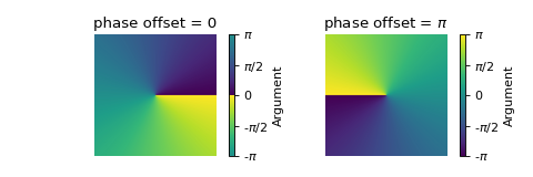

In the above figure, when using the HSV colormap the eye is drawn to the yellow, cyan and magenta colors, where there is a lightness gradient: those are false features caused by the colormap. Indeed, there is nothing going on these regions when looking with a perceptually uniform colormap.

Phase is computed with Numpy and lies between [-pi, pi]. Then, phase is normalized between [0, 1] using (arg / (2 * pi)) % 1. The figure below shows the mapping between phase in radians and normalized phase. A phase of 0 radians corresponds to a normalized phase of 0, which gets mapped to the beginning of a colormap.

(Source code, png)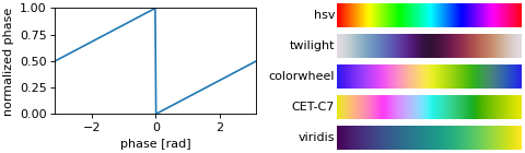

The zero radians phase is then located in the middle of the colorbar. Hence, the colorbar might feel “weird” if a sequential colormap is chosen, because there is a color-discontinuity in the middle of it, as can be seen in the previous example. The phaseoffset keyword argument allows to adjust the position of the colormap:

p1 = graphics(
    domain_coloring(z, (z, -2-2j, 2+2j), coloring="a",
        cmap="viridis", phaseoffset=0),
    grid=False, show=False, legend=True, aspect="equal",
    title="phase offset = 0", axis=False)
p2 = graphics(
    domain_coloring(z, (z, -2-2j, 2+2j), coloring="a",
        cmap="viridis", phaseoffset=pi),
    grid=False, show=False, legend=True, aspect="equal",
    title="phase offset = $\pi$", axis=False)
plotgrid(p1, p2, nc=2, size=(6, 2))

(Source code, png)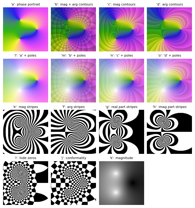

A pure phase portrait is rarely useful, as it conveys too little information. Let’s now quickly visualize the different coloring schemes. In the following, arg is the argument (phase), mag is the magnitude (absolute value) and contour is a line of constant value. Refer to [Wegert] for more information.

from matplotlib import rcParams
rcParams["font.size"] = 8
colorings = "abcdlmnoefghijk"
titles = [
    "phase portrait", "mag + arg contours", "mag contours", "arg contours",
    "'a' + poles", "'b' + poles", "'c' + poles", "'d' + poles",
    "mag stripes", "arg stripes", "real part stripes", "imag part stripes",
    "hide zeros", "conformality", "magnitude"]
plots = []
expr = (z - 1) / (z**2 + z + 1)
for c, t in zip(colorings, titles):
    plots.append(
        graphics(domain_coloring(expr, (z, -2-2j, 2+2j), coloring=c,
            cmap=colorcet.CET_C2, colorbar=False),
        grid=False, show=False, legend=False, axis=False,
        title=("'%s'" % c) + ": " + t, xlabel="", ylabel=""))

plotgrid(*plots, nc=4, size=(8, 8.5))

(Source code, png)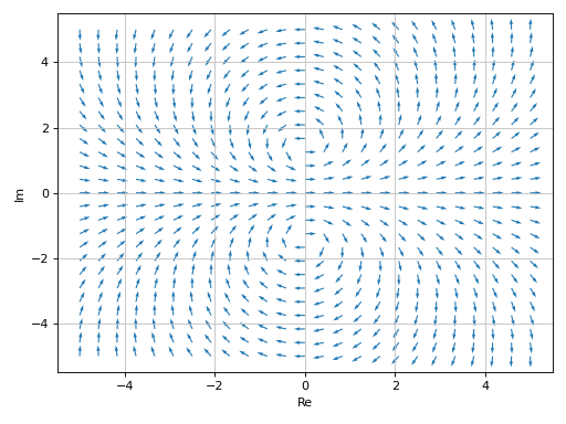

From the above picture, we can see that:

• Some enhancements decrese the lighness of the colors: depending on the colormap, it might be difficult to distinguish features in darker regions.

• Other enhancements increases the lightness in proximity of poles. Hence, colormaps with very light colors might not convey enough information.

With these considerations in mind, the selection of a proper colormap is left to the user because not only it depends on the target audience of the visualization, but also on the function being visualized.

Examples

>>> from sympy import I, symbols, exp, sqrt, cos, sin, pi, gamma
>>> from spb import *
>>> x, y, z = symbols('x, y, z')

(Source code)

To improve the smoothness of the results, increase the number of discretization points and/or apply an interpolation (if the backend supports it):

>>> graphics(
...     domain_coloring(gamma(z), (z, -3-3j, 3+3j), coloring="b", n=500),
...     grid=False)
Plot object containing:
[0]: complex domain coloring: gamma(z) for re(z) over (-3.0, 3.0) and im(z) over (-3.0, 3.0)

(Source code, png)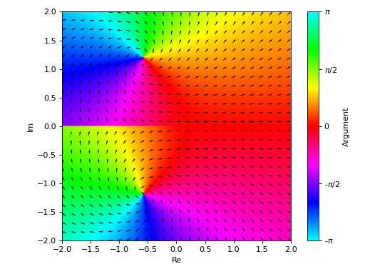

Use app=True to enable series-related widgets in order to quickly customize the appearance of the plot:

from sympy import *
from spb import *
z = symbols("z")
expr = (z - 1) / (z**2 + z + 2)
graphics(
    domain_coloring(expr, (z, -2-2j, 2+2j), n=500, coloring="b"),
    grid=False,
    app=True,
    template={"sidebar_width": "30%"},
    layout="sbl"
)

(Source code, small.png)

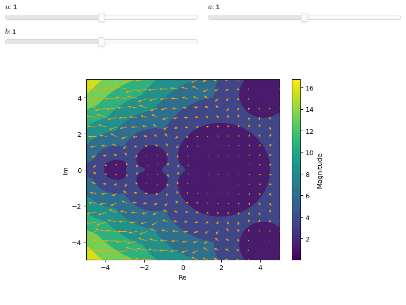
Interactive-widget domain coloring plot. Refer to the interactive sub-module documentation to learn more about the params dictionary. This plot illustrates:

• setting a custom colormap and adjusting the black-level of the enhanced visualization.

• the use of prange (parametric plotting range).

• the use of the params dictionary to specify sliders in their basic form: (default, min, max).

from sympy import *
from spb import *
import colorcet
z, u, a, b = symbols("z, u, a, b")
graphics(
    domain_coloring(sin(u * z), prange(z, -a - b*I, a + b*I),
        cmap=colorcet.colorwheel, blevel=0.85,
        coloring="b", n=250,
        params={
            u: (0.5, 0, 2),
            a: (pi, 0, 2*pi),
            b: (pi, 0, 2*pi),
        }),
    grid=False
)

(Source code, small.png)

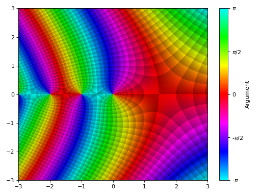
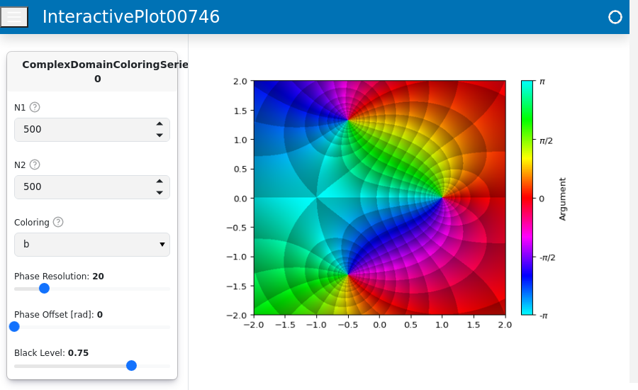
spb.graphics.complex_analysis.analytic_landscape(expr, range_c=None, label=None, rendering_kw=None, **kwargs)

Plot a surface of the absolute value of a complex function f(x) colored by its argument, with x in Complex.

Parameters:

expr

The expression representing the complex function to be plotted.

range_ctuple, Tuple

A 3-tuple (symb, min, max) denoting the range of the complex variable. Default values: min=-10-10j and max=10+10j.

labelstr

Set the label associated to this series, which will be eventually shown on the legend or colorbar.

rendering_kwdict

A dictionary of keyword arguments to be passed to the renderers in order to further customize the appearance of the line. Here are some useful links for the supported plotting libraries:

• Matplotlib: https://matplotlib.org/stable/api/_as_gen/matplotlib.pyplot.imshow.html

• Plotly: https://plotly.github.io/plotly.py-docs/generated/plotly.graph_objects.Image.html

• Bokeh: https://docs.bokeh.org/en/latest/docs/reference/models/glyphs/image_rgba.html#bokeh.models.ImageRGBA

annotatebool

Turn on/off the annotations on the 2D projections of the Riemann sphere. They can only be visible when riemann_mask=True. Default value: True.

at_infinitybool

If False the visualization will be centered about the complex point zero. Otherwise, it will be centered at infinity. Default value: False.

blevel

Controls the black level of ehanced domain coloring plots. It must be 0 (black) <= blevel <= 1 (white). It must be: 0 ≤ blevel ≤ 1. Default value: 0.75.

cmapstr, list, tuple

Specify the colormap to be used on enhanced domain coloring plots (both images and 3d plots). Default to "hsv". Can be any colormap from matplotlib or colorcet.

colorbarbool

Toggle the visibility of the colorbar associated to the current data series. Note that a colorbar is only visible if use_cm=True and color_func is not None. Default value: True.

colorbar_ticks_formattertick_formatter_multiples_of

An object of type tick_formatter_multiples_of which will be used to place tick values on the colorbar at each multiple of a specified quantity. This only works when use_cm=True.

coloringstr

Choose between different domain coloring options. Default to "a". Refer to [Wegert] for more information.

• "a": standard domain coloring showing the argument of the complex function.

• "b": enhanced domain coloring showing iso-modulus and iso-phase lines.

• "c": enhanced domain coloring showing iso-modulus lines.

• "d": enhanced domain coloring showing iso-phase lines.

• "e": alternating black and white stripes corresponding to modulus.

• "f": alternating black and white stripes corresponding to phase.

• "g": alternating black and white stripes corresponding to real part.

• "h": alternating black and white stripes corresponding to imaginary part.

• "i": cartesian chessboard on the complex points space. The result will hide zeros.

• "j": polar Chessboard on the complex points space. The result will show conformality.

• "k": black and white magnitude of the complex function. Zeros are black, poles are white.

• "k+log": same as "k" but apply a base 10 logarithm to the magnitude, which improves the visibility of zeros of functions with steep poles.

• "l":enhanced domain coloring showing iso-modulus and iso-phase lines, blended with the magnitude: white regions indicates greater magnitudes. Can be used to distinguish poles from zeros.

• "m": enhanced domain coloring showing iso-modulus lines, blended with the magnitude: white regions indicates greater magnitudes. Can be used to distinguish poles from zeros.

• "n": enhanced domain coloring showing iso-phase lines, blended with the magnitude: white regions indicates greater magnitudes. Can be used to distinguish poles from zeros.

• "o": enhanced domain coloring showing iso-phase lines, blended with the magnitude: white regions indicates greater magnitudes. Can be used to distinguish poles from zeros.

The user can also provide a callable, f(w), where w is an [n x m] Numpy array (provided by the plotting module) containing the results (complex numbers) of the evaluation of the complex function. The callable should return:

• imgndarray [n x m x 3]

  An array of RGB colors (0 <= R,G,B <= 255)

• colorscalendarray [N x 3] or None

  An array with N RGB colors, (0 <= R,G,B <= 255). If colorscale=None, no color bar will be shown on the plot.

Possible options: [‘a’, ‘b’, ‘c’, ‘d’, ‘e’, ‘f’, ‘g’, ‘h’, ‘i’, ‘j’, ‘k’, ‘k+log’, ‘l’, ‘m’, ‘n’, ‘o’] Default value: ‘a’.

force_real_evalbool

By default, numerical evaluation is performed over complex numbers, which is slower but produces correct results. However, when the symbolic expression is converted to a numerical function with lambdify, the resulting function may not like to be evaluated over complex numbers. In such cases, forcing the evaluation to be performed over real numbers might be a good choice. The plotting module should be able to detect such occurences and automatically activate this option. If that is not the case, or evaluation performance is of paramount importance, set this parameter to True, but be aware that it might produce wrong results. Default value: False.

modules

Specify the evaluation modules to be used by lambdify. If not specified, the evaluation will be done with NumPy/SciPy.

n1int

Number of discretization points along the x-axis (real part) to be used in the evaluation. Related parameters: xscale. It must be: 2 ≤ n1 < ∞. Default value: 300.

n2int

Number of discretization points along the y-axis (imaginary part) to be used in the evaluation. Related parameters: yscale. It must be: 2 ≤ n2 < ∞. Default value: 300.

only_integersbool

Discretize the domain using only integer numbers. When this parameter is True, the number of discretization points is choosen by the algorithm. Default value: False.

paramsdict, optional

A dictionary mapping symbols to parameters. If provided, this dictionary enables the interactive-widgets plot.

When calling a plotting function, the parameter can be specified with:

• a widget from the ipywidgets module.

• a widget from the panel module.

• a tuple of the form:

  (default, min, max, N, tick_format, label, spacing), which will instantiate a ipywidgets.widgets.widget_float.FloatSlider or a ipywidgets.widgets.widget_float.FloatLogSlider, depending on the spacing strategy. In particular:

  • default, min, maxfloat

    Default value, minimum value and maximum value of the slider, respectively. Must be finite numbers. The order of these 3 numbers is not important: the module will figure it out which is what.

  • Nint, optional

    Number of steps of the slider.

  • tick_formatstr or None, optional

    Provide a formatter for the tick value of the slider. Default to ".2f".

  • label: str, optional

    Custom text associated to the slider.

  • spacingstr, optional

    Specify the discretization spacing. Default to "linear", can be changed to "log".

Notes:

1. parameters cannot be linked together (ie, one parameter cannot depend on another one).

2. If a widget returns multiple numerical values (like panel.widgets.slider.RangeSlider or ipywidgets.widgets.widget_float.FloatRangeSlider), then a corresponding number of symbols must be provided.

Here follows a couple of examples. If imodule="panel":

import panel as pn
params = {
    a: (1, 0, 5), # slider from 0 to 5, with default value of 1
    b: pn.widgets.FloatSlider(value=1, start=0, end=5), # same slider as above
    (c, d): pn.widgets.RangeSlider(value=(-1, 1), start=-3, end=3, step=0.1)
}

Or with imodule="ipywidgets":

import ipywidgets as w
params = {
    a: (1, 0, 5), # slider from 0 to 5, with default value of 1
    b: w.FloatSlider(value=1, min=0, max=5), # same slider as above
    (c, d): w.FloatRangeSlider(value=(-1, 1), min=-3, max=3, step=0.1)
}

When instantiating a data series directly, params must be a dictionary mapping symbols to numerical values.

Let series be any data series. Then series.params returns a dictionary mapping symbols to numerical values.

phaseoffset

Controls the phase offset of the colormap in domain coloring plots. It must be: 0 ≤ phaseoffset ≤ 6.283185307179586. Default value: 0.

phaseresint

It controls the number of iso-phase and/or iso-modulus lines in domain coloring plots. It must be: 1 ≤ phaseres ≤ 100. Default value: 20.

riemann_maskbool

Turn on/off the unit disk mask representing the Riemann sphere on the 2D projections. Default value: False.

show_in_legendbool

Toggle the visibility of the data series on the legend. Default value: True.

sum_boundint

When plotting sums, the expression will be pre-processed in order to replace lower/upper bounds set to +/- infinity with this +/- numerical value. Note: the higher this number, the slower the evaluation, but the more accurate the plot. It must be: 0 ≤ sum_bound < ∞. Default value: 1000.

surface_color

For back-compatibility with old sympy.plotting. Use rendering_kw in order to fully customize the appearance of the surface.

txcallable

Numerical transformation function to be applied to the data on the x-axis.

tycallable

Numerical transformation function to be applied to the data on the y-axis.

tzcallable

Numerical transformation function to be applied to the data on the z-axis.

xscalestr

Discretization strategy along the x-direction (real part). Related parameters: n1. Possible options: [‘linear’, ‘log’] Default value: ‘linear’.

yscalestr

Discretization strategy along the y-direction (imaginary part). Related parameters: n12. Possible options: [‘linear’, ‘log’] Default value: ‘linear’.

Returns:

serieslist

A list containing up two to instance of ComplexDomainColoringSeries.

See also

domain_coloring

Examples

from sympy import symbols, gamma, I
from spb import *
z = symbols('z')
graphics(
    analytic_landscape(gamma(z), (z, -3 - 3*I, 3 + 3*I)),
    backend=PB, zlim=(-1, 6))

(Source code, png)

Because the function goes to infinity at poles, sometimes it might be beneficial to visualize the logarithm of the absolute value in order to easily identify zeros:

from sympy import symbols, I
from spb import *
import numpy as np
z = symbols("z")
expr = (z**3 - 5) / z
graphics(
    analytic_landscape(expr, (z, -3-3j, 3+3j), coloring="b", n=500,
        tz=np.log),
    grid=False, backend=KB)

(Source code, small.png)

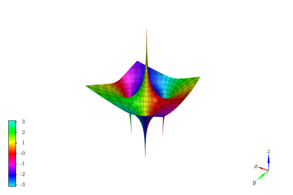
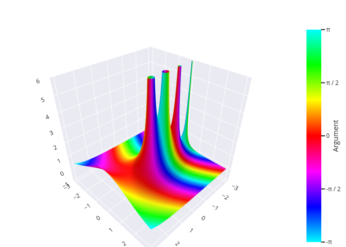
spb.graphics.complex_analysis.riemann_sphere_2d(expr, range_c=None, label=None, rendering_kw=None, at_infinity=False, riemann_mask=True, annotate=True, **kwargs)

Visualize stereographic projections of the Riemann sphere.

Refer to plot_riemann_sphere() to learn more about the Riemann sphere.

Parameters:

expr

The expression representing the complex function to be plotted.

range_ctuple, Tuple

A 3-tuple (symb, min, max) denoting the range of the complex variable. Default values: min=-10-10j and max=10+10j.

labelstr

Set the label associated to this series, which will be eventually shown on the legend or colorbar.

rendering_kwdict

A dictionary of keyword arguments to be passed to the renderers in order to further customize the appearance of the line. Here are some useful links for the supported plotting libraries:

• Matplotlib: https://matplotlib.org/stable/api/_as_gen/matplotlib.pyplot.imshow.html

• Plotly: https://plotly.github.io/plotly.py-docs/generated/plotly.graph_objects.Image.html

• Bokeh: https://docs.bokeh.org/en/latest/docs/reference/models/glyphs/image_rgba.html#bokeh.models.ImageRGBA

at_infinitybool

If False the visualization will be centered about the complex point zero. Otherwise, it will be centered at infinity. Default value: False.

riemann_maskbool

Turn on/off the unit disk mask representing the Riemann sphere on the 2D projections. Default value: False.

annotatebool

Turn on/off the annotations on the 2D projections of the Riemann sphere. They can only be visible when riemann_mask=True. Default value: True.

blevel

Controls the black level of ehanced domain coloring plots. It must be 0 (black) <= blevel <= 1 (white). It must be: 0 ≤ blevel ≤ 1. Default value: 0.75.

cmapstr, list, tuple

Specify the colormap to be used on enhanced domain coloring plots (both images and 3d plots). Default to "hsv". Can be any colormap from matplotlib or colorcet.

colorbarbool

Toggle the visibility of the colorbar associated to the current data series. Note that a colorbar is only visible if use_cm=True and color_func is not None. Default value: True.

colorbar_ticks_formattertick_formatter_multiples_of

An object of type tick_formatter_multiples_of which will be used to place tick values on the colorbar at each multiple of a specified quantity. This only works when use_cm=True.

coloringstr

Choose between different domain coloring options. Default to "a". Refer to [Wegert] for more information.

• "a": standard domain coloring showing the argument of the complex function.

• "b": enhanced domain coloring showing iso-modulus and iso-phase lines.

• "c": enhanced domain coloring showing iso-modulus lines.

• "d": enhanced domain coloring showing iso-phase lines.

• "e": alternating black and white stripes corresponding to modulus.

• "f": alternating black and white stripes corresponding to phase.

• "g": alternating black and white stripes corresponding to real part.

• "h": alternating black and white stripes corresponding to imaginary part.

• "i": cartesian chessboard on the complex points space. The result will hide zeros.

• "j": polar Chessboard on the complex points space. The result will show conformality.

• "k": black and white magnitude of the complex function. Zeros are black, poles are white.

• "k+log": same as "k" but apply a base 10 logarithm to the magnitude, which improves the visibility of zeros of functions with steep poles.

• "l":enhanced domain coloring showing iso-modulus and iso-phase lines, blended with the magnitude: white regions indicates greater magnitudes. Can be used to distinguish poles from zeros.

• "m": enhanced domain coloring showing iso-modulus lines, blended with the magnitude: white regions indicates greater magnitudes. Can be used to distinguish poles from zeros.

• "n": enhanced domain coloring showing iso-phase lines, blended with the magnitude: white regions indicates greater magnitudes. Can be used to distinguish poles from zeros.

• "o": enhanced domain coloring showing iso-phase lines, blended with the magnitude: white regions indicates greater magnitudes. Can be used to distinguish poles from zeros.

The user can also provide a callable, f(w), where w is an [n x m] Numpy array (provided by the plotting module) containing the results (complex numbers) of the evaluation of the complex function. The callable should return:

• imgndarray [n x m x 3]

  An array of RGB colors (0 <= R,G,B <= 255)

• colorscalendarray [N x 3] or None

  An array with N RGB colors, (0 <= R,G,B <= 255). If colorscale=None, no color bar will be shown on the plot.

Possible options: [‘a’, ‘b’, ‘c’, ‘d’, ‘e’, ‘f’, ‘g’, ‘h’, ‘i’, ‘j’, ‘k’, ‘k+log’, ‘l’, ‘m’, ‘n’, ‘o’] Default value: ‘a’.

force_real_evalbool

By default, numerical evaluation is performed over complex numbers, which is slower but produces correct results. However, when the symbolic expression is converted to a numerical function with lambdify, the resulting function may not like to be evaluated over complex numbers. In such cases, forcing the evaluation to be performed over real numbers might be a good choice. The plotting module should be able to detect such occurences and automatically activate this option. If that is not the case, or evaluation performance is of paramount importance, set this parameter to True, but be aware that it might produce wrong results. Default value: False.

modules

Specify the evaluation modules to be used by lambdify. If not specified, the evaluation will be done with NumPy/SciPy.

n1int

Number of discretization points along the x-axis (real part) to be used in the evaluation. Related parameters: xscale. It must be: 2 ≤ n1 < ∞. Default value: 300.

n2int

Number of discretization points along the y-axis (imaginary part) to be used in the evaluation. Related parameters: yscale. It must be: 2 ≤ n2 < ∞. Default value: 300.

only_integersbool

Discretize the domain using only integer numbers. When this parameter is True, the number of discretization points is choosen by the algorithm. Default value: False.

paramsdict, optional

A dictionary mapping symbols to parameters. If provided, this dictionary enables the interactive-widgets plot.

When calling a plotting function, the parameter can be specified with:

• a widget from the ipywidgets module.

• a widget from the panel module.

• a tuple of the form:

  (default, min, max, N, tick_format, label, spacing), which will instantiate a ipywidgets.widgets.widget_float.FloatSlider or a ipywidgets.widgets.widget_float.FloatLogSlider, depending on the spacing strategy. In particular:

  • default, min, maxfloat

    Default value, minimum value and maximum value of the slider, respectively. Must be finite numbers. The order of these 3 numbers is not important: the module will figure it out which is what.

  • Nint, optional

    Number of steps of the slider.

  • tick_formatstr or None, optional

    Provide a formatter for the tick value of the slider. Default to ".2f".

  • label: str, optional

    Custom text associated to the slider.

  • spacingstr, optional

    Specify the discretization spacing. Default to "linear", can be changed to "log".

Notes:

1. parameters cannot be linked together (ie, one parameter cannot depend on another one).

2. If a widget returns multiple numerical values (like panel.widgets.slider.RangeSlider or ipywidgets.widgets.widget_float.FloatRangeSlider), then a corresponding number of symbols must be provided.

Here follows a couple of examples. If imodule="panel":

import panel as pn
params = {
    a: (1, 0, 5), # slider from 0 to 5, with default value of 1
    b: pn.widgets.FloatSlider(value=1, start=0, end=5), # same slider as above
    (c, d): pn.widgets.RangeSlider(value=(-1, 1), start=-3, end=3, step=0.1)
}

Or with imodule="ipywidgets":

import ipywidgets as w
params = {
    a: (1, 0, 5), # slider from 0 to 5, with default value of 1
    b: w.FloatSlider(value=1, min=0, max=5), # same slider as above
    (c, d): w.FloatRangeSlider(value=(-1, 1), min=-3, max=3, step=0.1)
}

When instantiating a data series directly, params must be a dictionary mapping symbols to numerical values.

Let series be any data series. Then series.params returns a dictionary mapping symbols to numerical values.

phaseoffset

Controls the phase offset of the colormap in domain coloring plots. It must be: 0 ≤ phaseoffset ≤ 6.283185307179586. Default value: 0.

phaseresint

It controls the number of iso-phase and/or iso-modulus lines in domain coloring plots. It must be: 1 ≤ phaseres ≤ 100. Default value: 20.

show_in_legendbool

Toggle the visibility of the data series on the legend. Default value: True.

sum_boundint

When plotting sums, the expression will be pre-processed in order to replace lower/upper bounds set to +/- infinity with this +/- numerical value. Note: the higher this number, the slower the evaluation, but the more accurate the plot. It must be: 0 ≤ sum_bound < ∞. Default value: 1000.

surface_color

For back-compatibility with old sympy.plotting. Use rendering_kw in order to fully customize the appearance of the surface.

txcallable

Numerical transformation function to be applied to the data on the x-axis.

tycallable

Numerical transformation function to be applied to the data on the y-axis.

tzcallable

Numerical transformation function to be applied to the data on the z-axis.

xscalestr

Discretization strategy along the x-direction (real part). Related parameters: n1. Possible options: [‘linear’, ‘log’] Default value: ‘linear’.

yscalestr

Discretization strategy along the y-direction (imaginary part). Related parameters: n12. Possible options: [‘linear’, ‘log’] Default value: ‘linear’.

Returns:

serieslist

A list containing up two to instance of ComplexDomainColoringSeries.

See also

riemann_sphere_3d, domain_coloring

spb.plot_functions.complex_analysis.plot_riemann_sphere

Notes

plot_riemann_sphere() returns a plotgrid() of two visualizations, one with at_infinity=True, the other with at_infinity=False. Read its documentation to learn more about the [Riemann-sphere].

Examples

Visualization centerd at zero:

>>> from sympy import I, symbols, exp, sqrt, cos, sin, pi, gamma
>>> from spb import *
>>> z = symbols("z")
>>> expr = (z - 1) / (z**2 + z + 2)
>>> graphics(riemann_sphere_2d(expr, coloring="b", n=800), grid=False)
Plot object containing:
[0]: complex domain coloring: (z - 1)/(z**2 + z + 2) for re(z) over (-1.25, 1.25) and im(z) over (-1.25, 1.25)
[1]: parametric cartesian line: (cos(t), sin(t)) for t over (0, 2*pi)

(Source code, png)

Visualization centerd at infinity:

>>> graphics(riemann_sphere_2d(expr, coloring="b", n=800,
...     at_infinity=True), grid=False)
Plot object containing:
[0]: complex domain coloring: (-1 + 1/z)/(2 + 1/z + z**(-2)) for re(z) over (-1.25, 1.25) and im(z) over (-1.25, 1.25)
[1]: parametric cartesian line: (cos(t), sin(t)) for t over (0, 2*pi)

(Source code, png)

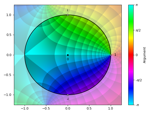
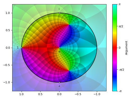
spb.graphics.complex_analysis.riemann_sphere_3d(expr, rendering_kw=None, colorbar=True, **kwargs)

Visualize a complex function over the Riemann sphere.

Parameters:

expr

The expression representing the complex function to be plotted.

rendering_kwdict

Keyword arguments to be passed to the renderers of the selected plotting library in order to further customize the appearance of this data series.

colorbarbool

Toggle the visibility of the colorbar associated to the current data series. Note that a colorbar is only visible if use_cm=True and color_func is not None. Default value: True.

blevel

Controls the black level of ehanced domain coloring plots. It must be 0 (black) <= blevel <= 1 (white). It must be: 0 ≤ blevel ≤ 1. Default value: 0.75.

cmapstr, list, tuple

Specify the colormap to be used on enhanced domain coloring plots (both images and 3d plots). Default to "hsv". Can be any colormap from matplotlib or colorcet.

coloringstr

Choose between different domain coloring options. Default to "a". Refer to [Wegert] for more information.

• "a": standard domain coloring showing the argument of the complex function.

• "b": enhanced domain coloring showing iso-modulus and iso-phase lines.

• "c": enhanced domain coloring showing iso-modulus lines.

• "d": enhanced domain coloring showing iso-phase lines.

• "e": alternating black and white stripes corresponding to modulus.

• "f": alternating black and white stripes corresponding to phase.

• "g": alternating black and white stripes corresponding to real part.

• "h": alternating black and white stripes corresponding to imaginary part.

• "i": cartesian chessboard on the complex points space. The result will hide zeros.

• "j": polar Chessboard on the complex points space. The result will show conformality.

• "k": black and white magnitude of the complex function. Zeros are black, poles are white.

• "k+log": same as "k" but apply a base 10 logarithm to the magnitude, which improves the visibility of zeros of functions with steep poles.

• "l":enhanced domain coloring showing iso-modulus and iso-phase lines, blended with the magnitude: white regions indicates greater magnitudes. Can be used to distinguish poles from zeros.

• "m": enhanced domain coloring showing iso-modulus lines, blended with the magnitude: white regions indicates greater magnitudes. Can be used to distinguish poles from zeros.

• "n": enhanced domain coloring showing iso-phase lines, blended with the magnitude: white regions indicates greater magnitudes. Can be used to distinguish poles from zeros.

• "o": enhanced domain coloring showing iso-phase lines, blended with the magnitude: white regions indicates greater magnitudes. Can be used to distinguish poles from zeros.

The user can also provide a callable, f(w), where w is an [n x m] Numpy array (provided by the plotting module) containing the results (complex numbers) of the evaluation of the complex function. The callable should return:

• imgndarray [n x m x 3]

  An array of RGB colors (0 <= R,G,B <= 255)

• colorscalendarray [N x 3] or None

  An array with N RGB colors, (0 <= R,G,B <= 255). If colorscale=None, no color bar will be shown on the plot.

Possible options: [‘a’, ‘b’, ‘c’, ‘d’, ‘e’, ‘f’, ‘g’, ‘h’, ‘i’, ‘j’, ‘k’, ‘k+log’, ‘l’, ‘m’, ‘n’, ‘o’] Default value: ‘a’.

labelstr

Set the label associated to this series, which will be eventually shown on the legend or colorbar.

n1int

Number of discretization points along the polar angle to be used in the evaluation. It must be: 2 ≤ n1 < ∞. Default value: 150.

n2int

Number of discretization points along the azimuthal angle to be used in the evaluation. It must be: 2 ≤ n2 < ∞. Default value: 600.

paramsdict, optional

A dictionary mapping symbols to parameters. If provided, this dictionary enables the interactive-widgets plot.

When calling a plotting function, the parameter can be specified with:

• a widget from the ipywidgets module.

• a widget from the panel module.

• a tuple of the form:

  (default, min, max, N, tick_format, label, spacing), which will instantiate a ipywidgets.widgets.widget_float.FloatSlider or a ipywidgets.widgets.widget_float.FloatLogSlider, depending on the spacing strategy. In particular:

  • default, min, maxfloat

    Default value, minimum value and maximum value of the slider, respectively. Must be finite numbers. The order of these 3 numbers is not important: the module will figure it out which is what.

  • Nint, optional

    Number of steps of the slider.

  • tick_formatstr or None, optional

    Provide a formatter for the tick value of the slider. Default to ".2f".

  • label: str, optional

    Custom text associated to the slider.

  • spacingstr, optional

    Specify the discretization spacing. Default to "linear", can be changed to "log".

Notes:

1. parameters cannot be linked together (ie, one parameter cannot depend on another one).

2. If a widget returns multiple numerical values (like panel.widgets.slider.RangeSlider or ipywidgets.widgets.widget_float.FloatRangeSlider), then a corresponding number of symbols must be provided.

Here follows a couple of examples. If imodule="panel":

import panel as pn
params = {
    a: (1, 0, 5), # slider from 0 to 5, with default value of 1
    b: pn.widgets.FloatSlider(value=1, start=0, end=5), # same slider as above
    (c, d): pn.widgets.RangeSlider(value=(-1, 1), start=-3, end=3, step=0.1)
}

Or with imodule="ipywidgets":

import ipywidgets as w
params = {
    a: (1, 0, 5), # slider from 0 to 5, with default value of 1
    b: w.FloatSlider(value=1, min=0, max=5), # same slider as above
    (c, d): w.FloatRangeSlider(value=(-1, 1), min=-3, max=3, step=0.1)
}

When instantiating a data series directly, params must be a dictionary mapping symbols to numerical values.

Let series be any data series. Then series.params returns a dictionary mapping symbols to numerical values.

phaseoffset

Controls the phase offset of the colormap in domain coloring plots. It must be: 0 ≤ phaseoffset ≤ 6.283185307179586. Default value: 0.

phaseresint

It controls the number of iso-phase and/or iso-modulus lines in domain coloring plots. It must be: 1 ≤ phaseres ≤ 100. Default value: 20.

range_ptuple, Tuple

A 3-tuple (symb, min, max) denoting the range of the azimuthal angle phi, usually ranging from [0, 2*pi]. Default values: min=-10 and max=10.

range_ttuple, Tuple

A 3-tuple (symb, min, max) denoting the range of the polar angle theta, usually ranging from [0, pi/2] for half hemisphere. Default values: min=-10 and max=10.

show_in_legendbool

Toggle the visibility of the data series on the legend. Default value: True.

txcallable

Numerical transformation function to be applied to the data on the x-axis.

tycallable

Numerical transformation function to be applied to the data on the y-axis.

tzcallable

Numerical transformation function to be applied to the data on the z-axis.

Returns:

serieslist

A list containing two to instance of RiemannSphereSeries.

See also

riemann_sphere_2d, domain_coloring

Examples

from sympy import *
from spb import *
z = symbols("z")
expr = (z - 1) / (z**2 + z + 1)
graphics(
    riemann_sphere_3d(expr, n=150,
        coloring="b"),
    backend=KB, legend=False, grid=False)

(Source code, small.png)

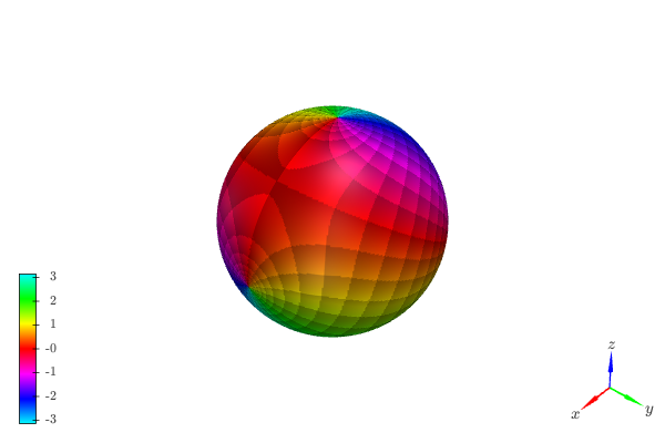
spb.graphics.complex_analysis.complex_vector_field(expr, range_c=None, **kwargs)

Plot the vector field [re(f), im(f)] for a complex function f over the specified complex domain.

Parameters:

exprExpr

Represent the complex function.

range_ctuple

A 3-element tuples denoting the range of the variables. For example (z, -5 - 3*I, 5 + 3*I). Note that we can specify the range by using standard Python complex numbers, for example (z, -5-3j, 5+3j).

color_func

Define the quiver/streamlines color mapping when use_cm=True. It can either be:

• A numerical function supporting vectorization. The arity must be: f(x, y, u, v). Further, scalar=False must be set in order to hide the contour plot so that a colormap is applied to quivers/streamlines.

• A symbolic expression having at most as many free symbols as u, v. This only works for quivers plot.

• None: the default value, which will map colors according to the magnitude of the vector field.

colorbarbool

Toggle the visibility of the colorbar associated to the current data series. Note that a colorbar is only visible if use_cm=True and color_func is not None. Default value: True.

force_real_evalbool

By default, numerical evaluation is performed over complex numbers, which is slower but produces correct results. However, when the symbolic expression is converted to a numerical function with lambdify, the resulting function may not like to be evaluated over complex numbers. In such cases, forcing the evaluation to be performed over real numbers might be a good choice. The plotting module should be able to detect such occurences and automatically activate this option. If that is not the case, or evaluation performance is of paramount importance, set this parameter to True, but be aware that it might produce wrong results. Default value: False.

is_streamlinesbool

If True shows the streamlines, otherwise visualize the vector field with quivers. Default value: False.

labelstr

Set the label associated to this series, which will be eventually shown on the legend or colorbar.

modules

Specify the evaluation modules to be used by lambdify. If not specified, the evaluation will be done with NumPy/SciPy.

n1int

Number of discretization points along the x-axis to be used in the evaluation. Related parameters: xscale. Default value: 25.

n2int

Number of discretization points along the y-axis to be used in the evaluation. Related parameters: yscale. Default value: 25.

normalizebool

If True, the vector field will be normalized, resulting in quivers having the same length. If use_cm=True, the backend will color the quivers by the (pre-normalized) vector field’s magnitude. Note: only quivers will be affected by this option.

Default value: False.

only_integersbool

Discretize the domain using only integer numbers. When this parameter is True, the number of discretization points is choosen by the algorithm. Default value: False.

paramsdict, optional

A dictionary mapping symbols to parameters. If provided, this dictionary enables the interactive-widgets plot.

When calling a plotting function, the parameter can be specified with:

• a widget from the ipywidgets module.

• a widget from the panel module.

• a tuple of the form:

  (default, min, max, N, tick_format, label, spacing), which will instantiate a ipywidgets.widgets.widget_float.FloatSlider or a ipywidgets.widgets.widget_float.FloatLogSlider, depending on the spacing strategy. In particular:

  • default, min, maxfloat

    Default value, minimum value and maximum value of the slider, respectively. Must be finite numbers. The order of these 3 numbers is not important: the module will figure it out which is what.

  • Nint, optional

    Number of steps of the slider.

  • tick_formatstr or None, optional

    Provide a formatter for the tick value of the slider. Default to ".2f".

  • label: str, optional

    Custom text associated to the slider.

  • spacingstr, optional

    Specify the discretization spacing. Default to "linear", can be changed to "log".

Notes:

1. parameters cannot be linked together (ie, one parameter cannot depend on another one).

2. If a widget returns multiple numerical values (like panel.widgets.slider.RangeSlider or ipywidgets.widgets.widget_float.FloatRangeSlider), then a corresponding number of symbols must be provided.

Here follows a couple of examples. If imodule="panel":

import panel as pn
params = {
    a: (1, 0, 5), # slider from 0 to 5, with default value of 1
    b: pn.widgets.FloatSlider(value=1, start=0, end=5), # same slider as above
    (c, d): pn.widgets.RangeSlider(value=(-1, 1), start=-3, end=3, step=0.1)
}

Or with imodule="ipywidgets":

import ipywidgets as w
params = {
    a: (1, 0, 5), # slider from 0 to 5, with default value of 1
    b: w.FloatSlider(value=1, min=0, max=5), # same slider as above
    (c, d): w.FloatRangeSlider(value=(-1, 1), min=-3, max=3, step=0.1)
}

When instantiating a data series directly, params must be a dictionary mapping symbols to numerical values.

Let series be any data series. Then series.params returns a dictionary mapping symbols to numerical values.

rendering_kwdict

A dictionary of keyword arguments to be passed to the renderers in order to further customize the appearance of the quivers or streamlines. Here are some useful links for the supported plotting libraries:

• Matplotlib:

  • quivers: https://matplotlib.org/stable/api/quiver_api.html#module-matplotlib.quiver

  • streamlines: https://matplotlib.org/stable/api/_as_gen/matplotlib.axes.Axes.streamplot.html#matplotlib.axes.Axes.streamplot

• Plotly:

  • 2D quivers: https://plotly.com/python/quiver-plots/

  • 2D streamlines: https://plotly.com/python/streamline-plots/

show_in_legendbool

Toggle the visibility of the data series on the legend. Default value: True.

sum_boundint

When plotting sums, the expression will be pre-processed in order to replace lower/upper bounds set to +/- infinity with this +/- numerical value. Note: the higher this number, the slower the evaluation, but the more accurate the plot. It must be: 0 ≤ sum_bound < ∞. Default value: 1000.

txcallable

Numerical transformation function to be applied to the data on the x-axis.

tycallable

Numerical transformation function to be applied to the data on the y-axis.

use_cmbool

Toggle the use of a colormap. By default, some series might use a colormap to display the necessary data. Setting this attribute to False will inform the associated renderer to use solid color. Related parameters: color_func. Default value: False.

xscalestr

Discretization strategy along the x-direction. Related parameters: n1. Possible options: [‘linear’, ‘log’] Default value: ‘linear’.

yscalestr

Discretization strategy along the y-direction. Related parameters: n2. Possible options: [‘linear’, ‘log’] Default value: ‘linear’.

Returns:

serieslist

A list containing one instance of ContourSeries (if scalar is set) and one instance of Vector2DSeries.

See also

spb.graphics.vectors.vector_field_2d

Examples

>>> from sympy import I, symbols, gamma, latex, log
>>> from spb import *
>>> z = symbols('z')

(Source code)

Quivers plot with normalize lengths and a contour plot in background representing the vector’s magnitude (a scalar field).

>>> expr = z**2 + 2
>>> graphics(
...     complex_vector_field(expr,  (z, -5 - 5j, 5 + 5j),
...         quiver_kw=dict(color="orange"), normalize=True,
...         contour_kw={"levels": 20}),
...     grid=False)
Plot object containing:
[0]: contour: sqrt(4*(re(_x) - im(_y))**2*(re(_y) + im(_x))**2 + ((re(_x) - im(_y))**2 - (re(_y) + im(_x))**2 + 2)**2) for _x over (-5.00000000000000, 5.00000000000000) and _y over (-5.00000000000000, 5.00000000000000)
[1]: 2D vector series: [(re(_x) - im(_y))**2 - (re(_y) + im(_x))**2 + 2, 2*(re(_x) - im(_y))*(re(_y) + im(_x))] over (_x, -5.0, 5.0), (_y, -5.0, 5.0)

(Source code, png)

Only quiver plot with normalized lengths and solid color.

>>> graphics(
...     complex_vector_field(expr,  (z, -5 - 5j, 5 + 5j),
...         scalar=False, use_cm=False, normalize=True),
...     grid=False, aspect="equal")
Plot object containing:
[0]: 2D vector series: [(re(_x) - im(_y))**2 - (re(_y) + im(_x))**2 + 2, 2*(re(_x) - im(_y))*(re(_y) + im(_x))] over (_x, -5.0, 5.0), (_y, -5.0, 5.0)

(Source code, png)

Only streamlines plot.

>>> graphics(
...     complex_vector_field(expr, (z, -5 - 5j, 5 + 5j),
...         label="Magnitude of $%s$" % latex(expr),
...         scalar=False, streamlines=True))
Plot object containing:
[0]: 2D vector series: [(re(_x) - im(_y))**2 - (re(_y) + im(_x))**2 + 2, 2*(re(_x) - im(_y))*(re(_y) + im(_x))] over (_x, -5.0, 5.0), (_y, -5.0, 5.0)

(Source code, png)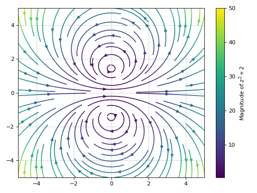

Overlay the quiver plot to a domain coloring plot. By setting n=26 (even number) in the complex vector plot, the quivers won’t to cross the branch cut.

>>> expr = z * log(2 * z) + 3
>>> graphics(
...     domain_coloring(expr, (z, -2-2j, 2+2j)),
...     complex_vector_field(expr, (z, -2-2j, 2+2j),
...         n=26, scalar=False, use_cm=False, normalize=True,
...         show_in_legend=False,
...         quiver_kw={"color": "k", "pivot": "tip"}),
...     grid=False)
Plot object containing:
[0]: complex domain coloring: z*log(2*z) + 3 for re(z) over (-2.0, 2.0) and im(z) over (-2.0, 2.0)
[1]: 2D vector series: [(re(_x) - im(_y))*log(Abs(2*_x + 2*_y*I)) - (re(_y) + im(_x))*arg(_x + _y*I) + 3, (re(_x) - im(_y))*arg(_x + _y*I) + (re(_y) + im(_x))*log(Abs(2*_x + 2*_y*I))] over (_x, -2.0, 2.0), (_y, -2.0, 2.0)

(Source code, png)

Interactive-widget plot. Refer to the interactive sub-module documentation to learn more about the params dictionary. This plot illustrates:

• the use of prange (parametric plotting range).

• the use of the params dictionary to specify sliders in their basic form: (default, min, max).

from sympy import *
from spb import *
z, u, a, b = symbols("z u a b")
graphics(
    complex_vector_field(
        log(gamma(u * z)), prange(z, -5*a - b*5j, 5*a + b*5j),
        params={
            u: (1, 0, 2),
            a: (1, 0, 2),
            b: (1, 0, 2)
        }, quiver_kw=dict(color="orange", headwidth=4)),
    n=20, grid=False)

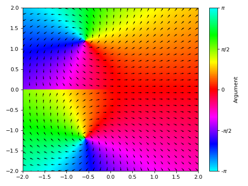
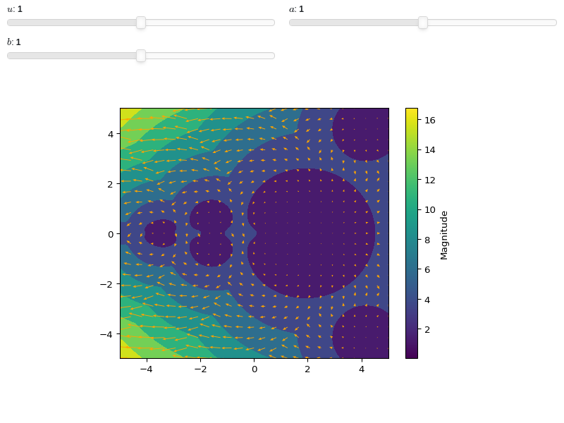(Source code, small.png)