2D general plotting
NOTE:
For technical reasons, all interactive-widgets plots in this documentation
are created using Holoviz’s Panel. Often, they will ran just fine with
ipywidgets too. However, if a specific example uses the param library,
or widgets from the panel module, then users will have to modify the
params dictionary in order to make it work with ipywidgets.
Refer to Interactive module for more information.
- spb.graphics.functions_2d.line(expr, range_x=None, label=None, rendering_kw=None, **kwargs)[source]
Plot a function of one variable over a 2D space.
- Parameters:
- expr
It can either be a symbolic expression representing the function of one variable to be plotted, or a numerical function of one variable, supporting vectorization. In the latter case the following keyword arguments are not supported:
params,sum_bound.- range_xtuple, Tuple
A 3-tuple (symb, min, max) denoting the range of the x variable. Default values: min=-10 and max=10.
- labelstr
Set the label associated to this series, which will be eventually shown on the legend or colorbar.
- rendering_kwdict
A dictionary of keyword arguments to be passed to the renderers in order to further customize the appearance of the line. Here are some useful links for the supported plotting libraries:
Matplotlib:
for solid lines: https://matplotlib.org/stable/api/_as_gen/matplotlib.pyplot.plot.html
for colormap-based lines: https://matplotlib.org/stable/api/collections_api.html#matplotlib.collections.LineCollection
for scatters: https://matplotlib.org/stable/api/_as_gen/matplotlib.pyplot.scatter.html
Bokeh:
- color_func
A color function to be applied to the numerical data. It can be:
A numerical function of 2 variables, x, y (the points computed by the internal algorithm) supporting vectorization.
A symbolic expression having at most as many free symbols as
expr.None: the default value (no color mapping).
- colorbarbool
Toggle the visibility of the colorbar associated to the current data series. Note that a colorbar is only visible if
use_cm=Trueandcolor_funcis not None. Default value: True.- colorbar_ticks_formattertick_formatter_multiples_of
An object of type
tick_formatter_multiples_ofwhich will be used to place tick values on the colorbar at each multiple of a specified quantity. This only works when use_cm=True.- detect_polesbool, str
Chose whether to detect and correctly plot the roots of the denominator. There are two algorithms at work:
based on the gradient of the numerical data, it introduces NaN values at locations where the steepness is greater than some threshold. This splits the line into multiple segments. To improve detection, increase the number of discretization points
nand/or change the value ofeps. This algorithm can be used to visualize jump discontinuities as well as essential discontinuities.a symbolic approach based on the
continuous_domainfunction from thesympy.calculus.utilmodule, which computes the locations of essential discontinuities. If any are found, vertical lines will be shown.
Possible options:
False: No poles detection
True: Poles detection with the numerical algorithm
‘symbolic’: Poles detection with numerical and symbolic algorithms
Default value: False.
- epsfloat
An arbitrary small value used by the
detect_polesnumerical algorithm. Before changing this value, it is recommended to increase the number of discretization points. Related parameters:detect_poles. It must be: 0 ≤ eps < ∞. Default value: 0.01.- excludelist
List of x-coordinates to be excluded from evaluation. In practice, it introduces discontinuities in the resulting line.
- force_real_evalbool
By default, numerical evaluation is performed over complex numbers, which is slower but produces correct results. However, when the symbolic expression is converted to a numerical function with lambdify, the resulting function may not like to be evaluated over complex numbers. In such cases, forcing the evaluation to be performed over real numbers might be a good choice. The plotting module should be able to detect such occurences and automatically activate this option. If that is not the case, or evaluation performance is of paramount importance, set this parameter to True, but be aware that it might produce wrong results. Default value: False.
- is_filledbool
Whether scatter’s markers are filled or void. Default value: True.
- is_scatterbool
If True it represent a scatter plot, otherwise a continuous line. Default value: False.
- line_color
For back-compatibility with old sympy.plotting. Use
rendering_kwin order to fully customize the appearance of the line/scatter.- modules
Specify the evaluation modules to be used by lambdify. If not specified, the evaluation will be done with NumPy/SciPy.
- n1int
Number of discretization points along the parameter to be used in the numerical evaluation. An alias of this parameter is
n. Related parameters:xscale. It must be: 2 ≤ n1 < ∞. Default value: 1000.- only_integersbool
Discretize the domain using only integer numbers. When this parameter is True, the number of discretization points is choosen by the algorithm. Default value: False.
- paramsdict, optional
A dictionary mapping symbols to parameters. If provided, this dictionary enables the interactive-widgets plot.
When calling a plotting function, the parameter can be specified with:
a widget from the
ipywidgetsmodule.a widget from the
panelmodule.- a tuple of the form:
(default, min, max, N, tick_format, label, spacing), which will instantiate a
ipywidgets.widgets.widget_float.FloatSlideror aipywidgets.widgets.widget_float.FloatLogSlider, depending on the spacing strategy. In particular:- default, min, maxfloat
Default value, minimum value and maximum value of the slider, respectively. Must be finite numbers. The order of these 3 numbers is not important: the module will figure it out which is what.
- Nint, optional
Number of steps of the slider.
- tick_formatstr or None, optional
Provide a formatter for the tick value of the slider. Default to
".2f".
- label: str, optional
Custom text associated to the slider.
- spacingstr, optional
Specify the discretization spacing. Default to
"linear", can be changed to"log".
Notes:
parameters cannot be linked together (ie, one parameter cannot depend on another one).
If a widget returns multiple numerical values (like
panel.widgets.slider.RangeSlideroripywidgets.widgets.widget_float.FloatRangeSlider), then a corresponding number of symbols must be provided.
Here follows a couple of examples. If
imodule="panel":import panel as pn params = { a: (1, 0, 5), # slider from 0 to 5, with default value of 1 b: pn.widgets.FloatSlider(value=1, start=0, end=5), # same slider as above (c, d): pn.widgets.RangeSlider(value=(-1, 1), start=-3, end=3, step=0.1) }
Or with
imodule="ipywidgets":import ipywidgets as w params = { a: (1, 0, 5), # slider from 0 to 5, with default value of 1 b: w.FloatSlider(value=1, min=0, max=5), # same slider as above (c, d): w.FloatRangeSlider(value=(-1, 1), min=-3, max=3, step=0.1) }
When instantiating a data series directly,
paramsmust be a dictionary mapping symbols to numerical values.Let
seriesbe any data series. Thenseries.paramsreturns a dictionary mapping symbols to numerical values.- poles_locationslist
When
detect_poles="symbolic", stores the location of the computed poles (essential discontinuities) so that they can be appropriately rendered.- poles_rendering_kwdict
Rendering kw used to customize the appearance of vertical lines representing essential discontinuities. Related parameters:
poles_locations.- show_in_legendbool
Toggle the visibility of the data series on the legend. Default value: True.
- stepsNoneType, bool, str
If set, it connects consecutive points with steps rather than straight segments. Possible options: [‘pre’, ‘post’, ‘mid’, True, False, None] Default value: False.
- sum_boundint
When plotting sums, the expression will be pre-processed in order to replace lower/upper bounds set to +/- infinity with this +/- numerical value. Note: the higher this number, the slower the evaluation, but the more accurate the plot. It must be: 0 ≤ sum_bound < ∞. Default value: 1000.
- txcallable
Numerical transformation function to be applied to the data on the x-axis.
- tycallable
Numerical transformation function to be applied to the data on the y-axis.
- unwrapbool, dict
Whether to use numpy.unwrap() on the computed coordinates in order to get rid of discontinuities. It can be:
False: do not use
np.unwrap().True: use
np.unwrap()with default keyword arguments.dictionary of keyword arguments passed to
np.unwrap().
- use_cmbool
Toggle the use of a colormap. By default, some series might use a colormap to display the necessary data. Setting this attribute to False will inform the associated renderer to use solid color. Related parameters:
color_func. Default value: False.- xscalestr
Discretization strategy along the x-direction. Related parameters:
n1. Possible options: [‘linear’, ‘log’] Default value: ‘linear’.
- Returns:
- serieslist
A list containing one instance of
LineOver1DRangeSeries.
See also
Examples
>>> from sympy import symbols, sin, pi, tan, exp, cos, log, floor
>>> from spb import *
>>> x, y = symbols('x, y')
Single Plot
>>> graphics(line(x**2, (x, -5, 5)))
Plot object containing:
[0]: cartesian line: x**2 for x over (-5, 5)
(
Source code,png)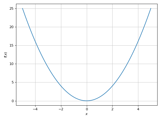
Multiple functions over the same range with custom rendering options:
>>> graphics(
...     line(x, (x, -3, 3)),
...     line(log(x), (x, -3, 3), rendering_kw={"linestyle": "--"}),
...     line(exp(x), (x, -3, 3), rendering_kw={"linestyle": ":"}),
...     aspect="equal", ylim=(-3, 3)
... )
Plot object containing:
[0]: cartesian line: x for x over (-3, 3)
[1]: cartesian line: log(x) for x over (-3, 3)
[2]: cartesian line: exp(x) for x over (-3, 3)
(
Source code,png)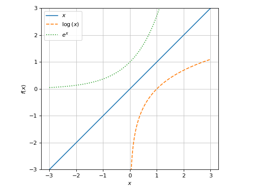
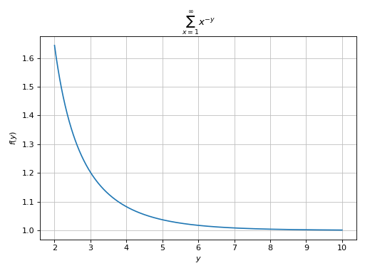
Plotting a summation in which the free symbol of the expression is not used in the lower/upper bounds:
>>> from sympy import Sum, oo, latex
>>> expr = Sum(1 / x ** y, (x, 1, oo))
>>> graphics(
...     line(expr, (y, 2, 10), sum_bound=1e03),
...     title="$%s$" % latex(expr)
... )
Plot object containing:
[0]: cartesian line: Sum(x**(-y), (x, 1, oo)) for y over (2, 10)
(
Source code,png)
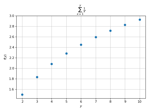
Plotting a summation in which the free symbol of the expression is used in the lower/upper bounds. Here, the discretization variable must assume integer values:
>>> expr = Sum(1 / x, (x, 1, y))
>>> graphics(
...     line(expr, (y, 2, 10), is_scatter=True),
...     title="$%s$" % latex(expr)
... )
Plot object containing:
[0]: cartesian line: Sum(1/x, (x, 1, y)) for y over (2, 10)
(
Source code,png)
Detect essential singularities and visualize them with vertical lines. Also, apply a tick formatter on the x-axis is order to show ticks at multiples of pi/2:
>>> import numpy as np
>>> graphics(
...     line(tan(x), (x, -1.5*pi, 1.5*pi), detect_poles="symbolic"),
...     x_ticks_formatter=multiples_of_pi_over_2(),
...     ylim=(-7, 7), xlabel="x [deg]", grid=False
... )
Plot object containing:
[0]: cartesian line: tan(x) for x over (-1.5*pi, 1.5*pi)
(
Source code,png)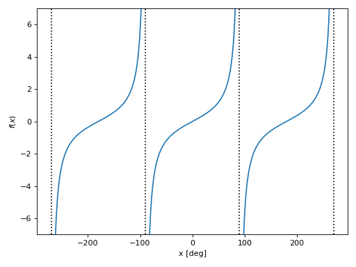
Introducing discontinuities by excluding specified points:
>>> graphics(
...     line(floor(x) / x, (x, -3.25, 3.25), exclude=list(range(-4, 5))),
...     ylim=(-1, 5)
... )
Plot object containing:
[0]: cartesian line: floor(x)/x for x over (-3.25000000000000, 3.25000000000000)
(
Source code,png)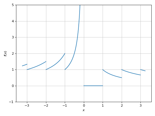
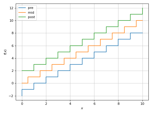
Creating a step plot:
>>> graphics(
...     line(x-2, (x, 0, 10), only_integers=True, steps="pre", label="pre"),
...     line(x, (x, 0, 10), only_integers=True, steps="mid", label="mid"),
...     line(x+2, (x, 0, 10), only_integers=True, steps="post", label="post"),
... )
Plot object containing:
[0]: cartesian line: x - 2 for x over (0, 10)
[1]: cartesian line: x for x over (0, 10)
[2]: cartesian line: x + 2 for x over (0, 10)
(
Source code,png)
Advanced example showing:
detect singularities by setting
adaptive=False(better performance), increasing the number of discretization points (in order to have ‘vertical’ segments on the lines) and reducing the threshold for the singularity-detection algorithm.application of color function.
combining together multiple lines.
>>> import numpy as np
>>> expr = 1 / cos(10 * x) + 5 * sin(x)
>>> def cf(x, y):
...     # map a colormap to the distance from the origin
...     d = np.sqrt(x**2 + y**2)
...     # visibility of the plot is limited: ylim=(-10, 10). However,
...     # some of the y-values computed by the function are much higher
...     # (or lower). Filter them out in order to have the entire
...     # colormap spectrum visible in the plot.
...     offset = 12 # 12 > 10 (safety margin)
...     d[(y > offset) | (y < -offset)] = 0
...     return d
>>> graphics(
...     line(
...         expr, (x, -5, 5), "distance from (0, 0)",
...         rendering_kw={"cmap": "plasma"},
...         adaptive=False, detect_poles=True, n=3e04,
...         eps=1e-04, color_func=cf),
...     line(5 * sin(x), (x, -5, 5), rendering_kw={"linestyle": "--"}),
...     ylim=(-10, 10), title="$%s$" % latex(expr)
... )
Plot object containing:
[0]: cartesian line: 5*sin(x) + 1/cos(10*x) for x over (-5, 5)
[1]: cartesian line: 5*sin(x) for x over (-5, 5)
(
Source code,png)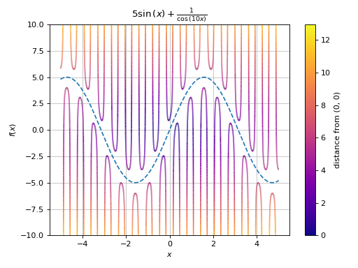
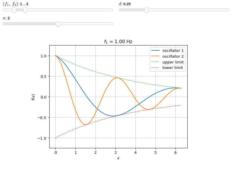
Interactive-widget plot of an oscillator. Refer to the interactive sub-module documentation to learn more about the
paramsdictionary. This plot illustrates:plotting multiple expressions, each one with its own label and rendering options.
the use of
prange(parametric plotting range).the use of the
paramsdictionary to specify sliders in their basic form: (default, min, max).the use of
panel.widgets.slider.RangeSlider, which is a 2-values widget. In this case it is used to enforce the condition f1 < f2.the use of a parametric title, specified with a tuple of the form:
(title_str, param_symbol1, ...), where:title_strmust be a formatted string, for example:"test = {:.2f}".param_symbol1, ...must be a symbol or a symbolic expression whose free symbols are contained in theparamsdictionary.
from sympy import *
from spb import *
import panel as pn
x, y, f1, f2, d, n = symbols("x, y, f_1, f_2, d, n")
params = {
    (f1, f2): pn.widgets.RangeSlider(
        value=(1, 2), start=0, end=10, step=0.1),     # frequencies
    d: (0.25, 0, 1),   # damping
    n: (2, 0, 4)       # multiple of pi
}
graphics(
    line(cos(f1 * x) * exp(-d * x), prange(x, 0, n * pi),
        label="oscillator 1", params=params),
    line(cos(f2 * x) * exp(-d * x), prange(x, 0, n * pi),
        label="oscillator 2", params=params),
    line(exp(-d * x), prange(x, 0, n * pi), label="upper limit",
        rendering_kw={"linestyle": ":"}, params=params),
    line(-exp(-d * x), prange(x, 0, n * pi), label="lower limit",
        rendering_kw={"linestyle": ":"}, params=params),
    ylim=(-1.25, 1.25),
    title=("$f_1$ = {:.2f} Hz", f1)
)
- spb.graphics.functions_2d.line_parametric_2d(expr_x, expr_y, range_p=None, label=None, rendering_kw=None, colorbar=True, use_cm=True, **kwargs)[source]
Plots a 2D parametric curve.
- Parameters:
- expr_x
The expression representing the component along the x-axis of the parametric function. It can either be a symbolic expression representing the function of one variable to be plotted, or a numerical function of one variable, supporting vectorization. In the latter case the following keyword arguments are not supported:
params,sum_bound.- expr_y
The expression representing the component along the y-axis of the parametric function. It can either be a symbolic expression representing the function of one variable to be plotted, or a numerical function of one variable, supporting vectorization. In the latter case the following keyword arguments are not supported:
params,sum_bound.- range_ptuple, Tuple
A 3-tuple (symb, min, max) denoting the range of the parameter. Default values: min=-10 and max=10.
- labelstr
Set the label associated to this series, which will be eventually shown on the legend or colorbar.
- rendering_kwdict
A dictionary of keyword arguments to be passed to the renderers in order to further customize the appearance of the line. Here are some useful links for the supported plotting libraries:
Matplotlib:
for solid lines: https://matplotlib.org/stable/api/_as_gen/matplotlib.pyplot.plot.html
for colormap-based lines: https://matplotlib.org/stable/api/collections_api.html#matplotlib.collections.LineCollection
for scatters: https://matplotlib.org/stable/api/_as_gen/matplotlib.pyplot.scatter.html
Bokeh:
- colorbarbool
Toggle the visibility of the colorbar associated to the current data series. Note that a colorbar is only visible if
use_cm=Trueandcolor_funcis not None. Default value: True.- use_cmbool
Toggle the use of a colormap. By default, some series might use a colormap to display the necessary data. Setting this attribute to False will inform the associated renderer to use solid color. Related parameters:
color_func. Default value: False.- color_func
Define a custom color mapping when
use_cm=True. It can either be:A numerical function supporting vectorization. The arity can be:
1 argument:
f(t), wheretis the parameter.2 arguments:
f(x, y)wherex, yare the coordinates of the points.3 arguments:
f(x, y, t).
A symbolic expression having at most as many free symbols as
expr_xorexpr_y.None: the default value (color mapping according to the parameter).
Alias of this parameters:
tp.- colorbar_ticks_formattertick_formatter_multiples_of
An object of type
tick_formatter_multiples_ofwhich will be used to place tick values on the colorbar at each multiple of a specified quantity. This only works when use_cm=True.- detect_polesbool, str
Chose whether to detect and correctly plot the roots of the denominator. There are two algorithms at work:
based on the gradient of the numerical data, it introduces NaN values at locations where the steepness is greater than some threshold. This splits the line into multiple segments. To improve detection, increase the number of discretization points
nand/or change the value ofeps. This algorithm can be used to visualize jump discontinuities as well as essential discontinuities.a symbolic approach based on the
continuous_domainfunction from thesympy.calculus.utilmodule, which computes the locations of essential discontinuities. If any are found, vertical lines will be shown.
Possible options:
False: No poles detection
True: Poles detection with the numerical algorithm
‘symbolic’: Poles detection with numerical and symbolic algorithms
Default value: False.
- epsfloat
An arbitrary small value used by the
detect_polesnumerical algorithm. Before changing this value, it is recommended to increase the number of discretization points. Related parameters:detect_poles. It must be: 0 ≤ eps < ∞. Default value: 0.01.- excludelist
A list of numerical values along the parameter which are going to be excluded from the evaluation. In practice, it introduces discontinuities in the resulting line.
- force_real_evalbool
By default, numerical evaluation is performed over complex numbers, which is slower but produces correct results. However, when the symbolic expression is converted to a numerical function with lambdify, the resulting function may not like to be evaluated over complex numbers. In such cases, forcing the evaluation to be performed over real numbers might be a good choice. The plotting module should be able to detect such occurences and automatically activate this option. If that is not the case, or evaluation performance is of paramount importance, set this parameter to True, but be aware that it might produce wrong results. Default value: False.
- is_filledbool
Whether scatter’s markers are filled or void. Default value: True.
- is_scatterbool
If True it represent a scatter plot, otherwise a continuous line. Default value: False.
- line_color
For back-compatibility with old sympy.plotting. Use
rendering_kwin order to fully customize the appearance of the line/scatter.- modules
Specify the evaluation modules to be used by lambdify. If not specified, the evaluation will be done with NumPy/SciPy.
- n1int
Number of discretization points along the parameter to be used in the evaluation. An alias of this parameter is
n. Related parameters:xscale. It must be: 2 ≤ n1 < ∞. Default value: 1000.- only_integersbool
Discretize the domain using only integer numbers. When this parameter is True, the number of discretization points is choosen by the algorithm. Default value: False.
- paramsdict, optional
A dictionary mapping symbols to parameters. If provided, this dictionary enables the interactive-widgets plot.
When calling a plotting function, the parameter can be specified with:
a widget from the
ipywidgetsmodule.a widget from the
panelmodule.- a tuple of the form:
(default, min, max, N, tick_format, label, spacing), which will instantiate a
ipywidgets.widgets.widget_float.FloatSlideror aipywidgets.widgets.widget_float.FloatLogSlider, depending on the spacing strategy. In particular:- default, min, maxfloat
Default value, minimum value and maximum value of the slider, respectively. Must be finite numbers. The order of these 3 numbers is not important: the module will figure it out which is what.
- Nint, optional
Number of steps of the slider.
- tick_formatstr or None, optional
Provide a formatter for the tick value of the slider. Default to
".2f".
- label: str, optional
Custom text associated to the slider.
- spacingstr, optional
Specify the discretization spacing. Default to
"linear", can be changed to"log".
Notes:
parameters cannot be linked together (ie, one parameter cannot depend on another one).
If a widget returns multiple numerical values (like
panel.widgets.slider.RangeSlideroripywidgets.widgets.widget_float.FloatRangeSlider), then a corresponding number of symbols must be provided.
Here follows a couple of examples. If
imodule="panel":import panel as pn params = { a: (1, 0, 5), # slider from 0 to 5, with default value of 1 b: pn.widgets.FloatSlider(value=1, start=0, end=5), # same slider as above (c, d): pn.widgets.RangeSlider(value=(-1, 1), start=-3, end=3, step=0.1) }
Or with
imodule="ipywidgets":import ipywidgets as w params = { a: (1, 0, 5), # slider from 0 to 5, with default value of 1 b: w.FloatSlider(value=1, min=0, max=5), # same slider as above (c, d): w.FloatRangeSlider(value=(-1, 1), min=-3, max=3, step=0.1) }
When instantiating a data series directly,
paramsmust be a dictionary mapping symbols to numerical values.Let
seriesbe any data series. Thenseries.paramsreturns a dictionary mapping symbols to numerical values.- show_in_legendbool
Toggle the visibility of the data series on the legend. Default value: True.
- sum_boundint
When plotting sums, the expression will be pre-processed in order to replace lower/upper bounds set to +/- infinity with this +/- numerical value. Note: the higher this number, the slower the evaluation, but the more accurate the plot. It must be: 0 ≤ sum_bound < ∞. Default value: 1000.
- txcallable
Numerical transformation function to be applied to the data on the x-axis.
- tycallable
Numerical transformation function to be applied to the data on the y-axis.
- xscalestr
Discretization strategy along the parameter. Possible options: [‘linear’, ‘log’] Default value: ‘linear’.
- Returns:
- serieslist
A list containing one instance of
Parametric2DLineSeries.
Examples
>>> from sympy import symbols, cos, sin, pi, floor, log
>>> from spb import *
>>> t, u, v = symbols('t, u, v')
A parametric plot of a single expression (a Hypotrochoid using an equal aspect ratio), showing colorbar’s ticks at multiple of pi:
>>> graphics(
...     line_parametric_2d(
...         2 * cos(u) + 5 * cos(2 * u / 3),
...         2 * sin(u) - 5 * sin(2 * u / 3),
...         (u, 0, 6 * pi),
...         colorbar_ticks_formatter=multiples_of_pi(),
...     ),
...     aspect="equal"
... )
Plot object containing:
[0]: parametric cartesian line: (5*cos(2*u/3) + 2*cos(u), -5*sin(2*u/3) + 2*sin(u)) for u over (0, 6*pi)
(
Source code,png)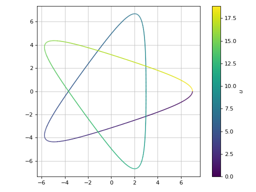
A parametric plot with multiple expressions with the same range with solid line colors:
>>> graphics(
...     line_parametric_2d(2 * cos(t), sin(t), (t, 0, 2*pi), use_cm=False),
...     line_parametric_2d(cos(t), 2 * sin(t), (t, 0, 2*pi), use_cm=False),
... )
Plot object containing:
[0]: parametric cartesian line: (2*cos(t), sin(t)) for t over (0, 2*pi)
[1]: parametric cartesian line: (cos(t), 2*sin(t)) for t over (0, 2*pi)
(
Source code,png)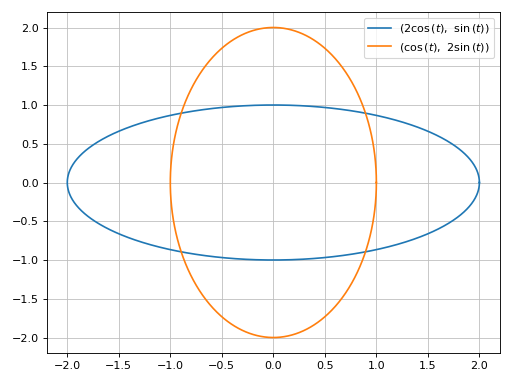
A parametric plot with multiple expressions with different ranges, custom labels, custom rendering options and a transformation function applied to the discretized parameter to convert radians to degrees:
>>> import numpy as np
>>> graphics(
...     line_parametric_2d(
...         3 * cos(u), 3 * sin(u), (u, 0, 2 * pi), "u [deg]",
...         rendering_kw={"lw": 3}, tp=np.rad2deg),
...     line_parametric_2d(
...         3 * cos(2 * v), 5 * sin(4 * v), (v, 0, pi), "v [deg]",
...         tp=np.rad2deg
...     ),
...     aspect="equal"
... )
Plot object containing:
[0]: parametric cartesian line: (3*cos(u), 3*sin(u)) for u over (0, 2*pi)
[1]: parametric cartesian line: (3*cos(2*v), 5*sin(4*v)) for v over (0, pi)
(
Source code,png)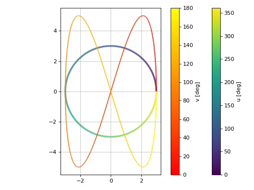
Introducing discontinuities by excluding specified points:
>>> e1 = log(floor(t))*cos(t)
>>> e2 = log(floor(t))*sin(t)
>>> graphics(
...     line_parametric_2d(
...         e1, e2, (t, 1, 4*pi), exclude=list(range(1, 13))),
...     grid=False
... )
Plot object containing:
[0]: parametric cartesian line: (log(floor(t))*cos(t), log(floor(t))*sin(t)) for t over (1, 4*pi)
(
Source code,png)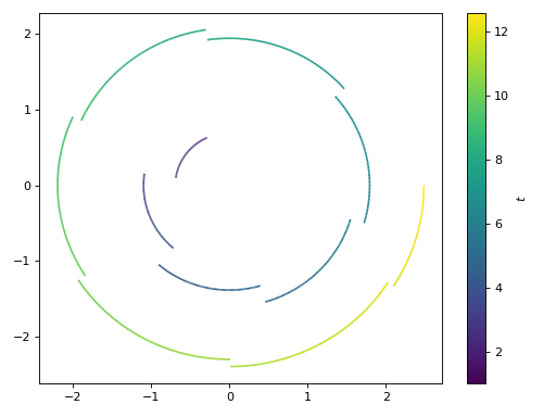
Plotting a numerical function instead of a symbolic expression:
>>> import numpy as np
>>> fx = lambda t: np.sin(t) * (np.exp(np.cos(t)) - 2 * np.cos(4 * t) - np.sin(t / 12)**5)
>>> fy = lambda t: np.cos(t) * (np.exp(np.cos(t)) - 2 * np.cos(4 * t) - np.sin(t / 12)**5)
>>> graphics(
...     line_parametric_2d(fx, fy, ("t", 0, 12 * pi),
...         use_cm=False, n=2000),
...     title="Butterfly Curve",
... )
(
Source code,png)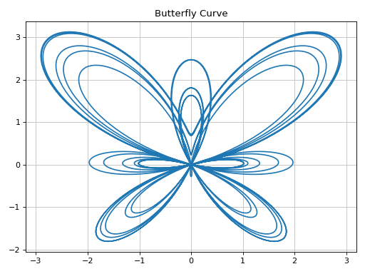
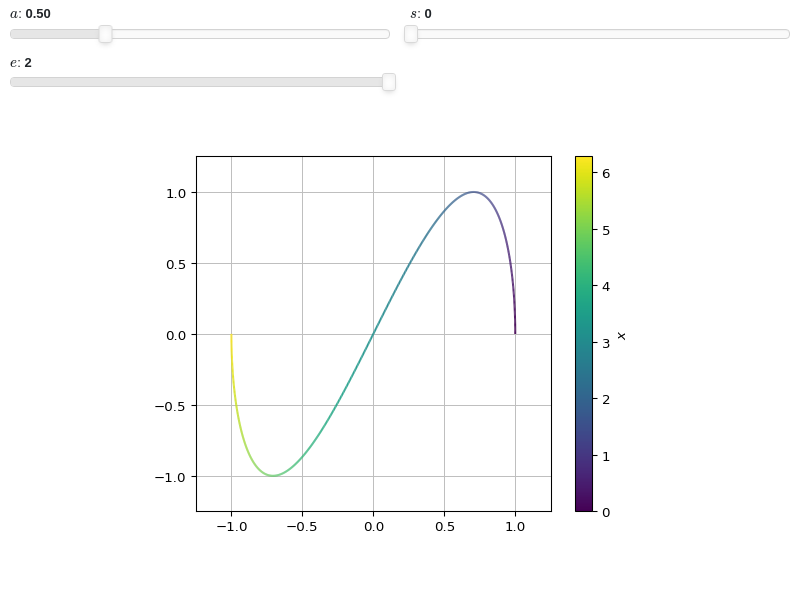
Interactive-widget plot. Refer to the interactive sub-module documentation to learn more about the
paramsdictionary. This plot illustrates:the use of
prange(parametric plotting range).the use of the
paramsdictionary to specify sliders in their basic form: (default, min, max).
from sympy import *
from spb import *
x, a, s, e = symbols("x a s, e")
graphics(
    line_parametric_2d(
        cos(a * x), sin(x), prange(x, s*pi, e*pi),
            params={
            a: (0.5, 0, 2),
            s: (0, 0, 2),
            e: (2, 0, 2),
        }),
    aspect="equal",
    xlim=(-1.25, 1.25), ylim=(-1.25, 1.25)
)
- spb.graphics.functions_2d.line_polar(expr, range_p=None, label=None, rendering_kw=None, **kwargs)[source]
Creates a 2D polar plot of a function of one variable.
- Parameters:
- range_ptuple, Tuple
A 3-tuple (symb, min, max) denoting the range of the parameter. Default values: min=-10 and max=10.
- labelstr
Set the label associated to this series, which will be eventually shown on the legend or colorbar.
- rendering_kwdict
A dictionary of keyword arguments to be passed to the renderers in order to further customize the appearance of the line. Here are some useful links for the supported plotting libraries:
Matplotlib:
for solid lines: https://matplotlib.org/stable/api/_as_gen/matplotlib.pyplot.plot.html
for colormap-based lines: https://matplotlib.org/stable/api/collections_api.html#matplotlib.collections.LineCollection
for scatters: https://matplotlib.org/stable/api/_as_gen/matplotlib.pyplot.scatter.html
Bokeh:
- color_func
Define a custom color mapping when
use_cm=True. It can either be:A numerical function supporting vectorization. The arity can be:
1 argument:
f(t), wheretis the parameter.2 arguments:
f(x, y)wherex, yare the coordinates of the points.3 arguments:
f(x, y, t).
A symbolic expression having at most as many free symbols as
expr_xorexpr_y.None: the default value (color mapping according to the parameter).
Alias of this parameters:
tp.- colorbarbool
Toggle the visibility of the colorbar associated to the current data series. Note that a colorbar is only visible if
use_cm=Trueandcolor_funcis not None. Default value: True.- colorbar_ticks_formattertick_formatter_multiples_of
An object of type
tick_formatter_multiples_ofwhich will be used to place tick values on the colorbar at each multiple of a specified quantity. This only works when use_cm=True.- detect_polesbool, str
Chose whether to detect and correctly plot the roots of the denominator. There are two algorithms at work:
based on the gradient of the numerical data, it introduces NaN values at locations where the steepness is greater than some threshold. This splits the line into multiple segments. To improve detection, increase the number of discretization points
nand/or change the value ofeps. This algorithm can be used to visualize jump discontinuities as well as essential discontinuities.a symbolic approach based on the
continuous_domainfunction from thesympy.calculus.utilmodule, which computes the locations of essential discontinuities. If any are found, vertical lines will be shown.
Possible options:
False: No poles detection
True: Poles detection with the numerical algorithm
‘symbolic’: Poles detection with numerical and symbolic algorithms
Default value: False.
- epsfloat
An arbitrary small value used by the
detect_polesnumerical algorithm. Before changing this value, it is recommended to increase the number of discretization points. Related parameters:detect_poles. It must be: 0 ≤ eps < ∞. Default value: 0.01.- excludelist
A list of numerical values along the parameter which are going to be excluded from the evaluation. In practice, it introduces discontinuities in the resulting line.
- expr_x
The expression representing the component along the x-axis of the parametric function. It can either be a symbolic expression representing the function of one variable to be plotted, or a numerical function of one variable, supporting vectorization. In the latter case the following keyword arguments are not supported:
params,sum_bound.- expr_y
The expression representing the component along the y-axis of the parametric function. It can either be a symbolic expression representing the function of one variable to be plotted, or a numerical function of one variable, supporting vectorization. In the latter case the following keyword arguments are not supported:
params,sum_bound.- force_real_evalbool
By default, numerical evaluation is performed over complex numbers, which is slower but produces correct results. However, when the symbolic expression is converted to a numerical function with lambdify, the resulting function may not like to be evaluated over complex numbers. In such cases, forcing the evaluation to be performed over real numbers might be a good choice. The plotting module should be able to detect such occurences and automatically activate this option. If that is not the case, or evaluation performance is of paramount importance, set this parameter to True, but be aware that it might produce wrong results. Default value: False.
- is_filledbool
Whether scatter’s markers are filled or void. Default value: True.
- is_scatterbool
If True it represent a scatter plot, otherwise a continuous line. Default value: False.
- line_color
For back-compatibility with old sympy.plotting. Use
rendering_kwin order to fully customize the appearance of the line/scatter.- modules
Specify the evaluation modules to be used by lambdify. If not specified, the evaluation will be done with NumPy/SciPy.
- n1int
Number of discretization points along the parameter to be used in the evaluation. An alias of this parameter is
n. Related parameters:xscale. It must be: 2 ≤ n1 < ∞. Default value: 1000.- only_integersbool
Discretize the domain using only integer numbers. When this parameter is True, the number of discretization points is choosen by the algorithm. Default value: False.
- paramsdict, optional
A dictionary mapping symbols to parameters. If provided, this dictionary enables the interactive-widgets plot.
When calling a plotting function, the parameter can be specified with:
a widget from the
ipywidgetsmodule.a widget from the
panelmodule.- a tuple of the form:
(default, min, max, N, tick_format, label, spacing), which will instantiate a
ipywidgets.widgets.widget_float.FloatSlideror aipywidgets.widgets.widget_float.FloatLogSlider, depending on the spacing strategy. In particular:- default, min, maxfloat
Default value, minimum value and maximum value of the slider, respectively. Must be finite numbers. The order of these 3 numbers is not important: the module will figure it out which is what.
- Nint, optional
Number of steps of the slider.
- tick_formatstr or None, optional
Provide a formatter for the tick value of the slider. Default to
".2f".
- label: str, optional
Custom text associated to the slider.
- spacingstr, optional
Specify the discretization spacing. Default to
"linear", can be changed to"log".
Notes:
parameters cannot be linked together (ie, one parameter cannot depend on another one).
If a widget returns multiple numerical values (like
panel.widgets.slider.RangeSlideroripywidgets.widgets.widget_float.FloatRangeSlider), then a corresponding number of symbols must be provided.
Here follows a couple of examples. If
imodule="panel":import panel as pn params = { a: (1, 0, 5), # slider from 0 to 5, with default value of 1 b: pn.widgets.FloatSlider(value=1, start=0, end=5), # same slider as above (c, d): pn.widgets.RangeSlider(value=(-1, 1), start=-3, end=3, step=0.1) }
Or with
imodule="ipywidgets":import ipywidgets as w params = { a: (1, 0, 5), # slider from 0 to 5, with default value of 1 b: w.FloatSlider(value=1, min=0, max=5), # same slider as above (c, d): w.FloatRangeSlider(value=(-1, 1), min=-3, max=3, step=0.1) }
When instantiating a data series directly,
paramsmust be a dictionary mapping symbols to numerical values.Let
seriesbe any data series. Thenseries.paramsreturns a dictionary mapping symbols to numerical values.- show_in_legendbool
Toggle the visibility of the data series on the legend. Default value: True.
- sum_boundint
When plotting sums, the expression will be pre-processed in order to replace lower/upper bounds set to +/- infinity with this +/- numerical value. Note: the higher this number, the slower the evaluation, but the more accurate the plot. It must be: 0 ≤ sum_bound < ∞. Default value: 1000.
- txcallable
Numerical transformation function to be applied to the data on the x-axis.
- tycallable
Numerical transformation function to be applied to the data on the y-axis.
- use_cmbool
Toggle the use of a colormap. By default, some series might use a colormap to display the necessary data. Setting this attribute to False will inform the associated renderer to use solid color. Related parameters:
color_func. Default value: False.- xscalestr
Discretization strategy along the parameter. Possible options: [‘linear’, ‘log’] Default value: ‘linear’.
See also
Examples
>>> from sympy import symbols, sin, cos, exp, pi
>>> from spb import *
>>> theta = symbols('theta')
Plot with cartesian axis:
>>> graphics(
...     line_polar(3 * sin(2 * theta), (theta, 0, 2*pi)),
...     aspect="equal"
... )
Plot object containing:
[0]: parametric cartesian line: (3*sin(2*theta)*cos(theta), 3*sin(theta)*sin(2*theta)) for theta over (0, 2*pi)
(
Source code,png)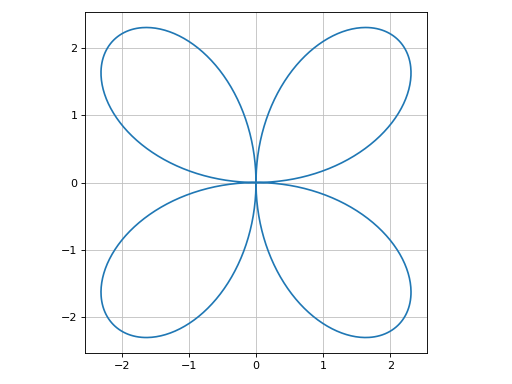
Plot with polar axis:
>>> graphics(
...     line_polar(exp(sin(theta)) - 2 * cos(4 * theta), (theta, 0, 2 * pi)),
...     polar_axis=True, aspect="equal"
... )
Plot object containing:
[0]: parametric cartesian line: ((exp(sin(theta)) - 2*cos(4*theta))*cos(theta), (exp(sin(theta)) - 2*cos(4*theta))*sin(theta)) for theta over (0, 2*pi)
(
Source code,png)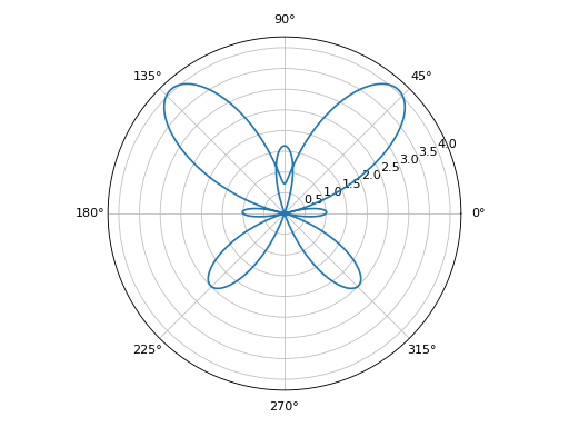
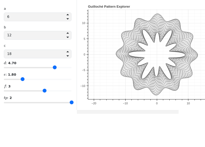
Interactive-widget plot of Guilloché Pattern. Refer to the interactive sub-module documentation to learn more about the
paramsdictionary. This plot illustrates:the use of
prange(parametric plotting range).the use of the
paramsdictionary to specify the widgets to be created by Holoviz’s Panel.
from sympy import *
from spb import *
import panel as pn
a, b, c, d, e, f, theta, tp = symbols("a:f theta tp")
def func(n):
    t1 = (c + sin(a * theta + d))
    t2 = ((b + sin(b * theta + e)) - (c + sin(a * theta + d)))
    t3 = (f + sin(a * theta + n / pi))
    return t1 + t2 * t3 / 2
params = {
    a: pn.widgets.IntInput(value=6, name="a"),
    b: pn.widgets.IntInput(value=12, name="b"),
    c: pn.widgets.IntInput(value=18, name="c"),
    d: (4.7, 0, 2*pi),
    e: (1.8, 0, 2*pi),
    f: (3, 0, 5),
    tp: (2, 0, 2)
}
series = []
for n in range(20):
    series += line_polar(
        func(n), prange(theta, 0, tp*pi), params=params,
        rendering_kw={"line_color": "black", "line_width": 0.5})
graphics(
    *series,
    aspect="equal",
    layout = "sbl",
    ncols = 1,
    title="Guilloché Pattern Explorer",
    backend=BB,
    legend=False,
    servable=True,
    imodule="panel"
)
- spb.graphics.functions_2d.contour(expr, range_x=None, range_y=None, label=None, rendering_kw=None, colorbar=True, clabels=True, fill=True, **kwargs)[source]
Plots contour lines or filled contours of a function of two variables.
- Parameters:
- expr
The expression representing the function of two variables to be plotted. It can be a:
Symbolic expression.
Numerical function of two variable, supporting vectorization. In this case the following keyword arguments are not supported:
params.
- range_xtuple, Tuple
A 3-tuple (symb, min, max) denoting the range of the x variable. Default values: min=-10 and max=10.
- range_ytuple, Tuple
A 3-tuple (symb, min, max) denoting the range of the y variable. Default values: min=-10 and max=10.
- labelstr
Set the label associated to this series, which will be eventually shown on the legend or colorbar.
- rendering_kwdict
A dictionary of keyword arguments to be passed to the renderers in order to further customize the appearance of the contour. Here are some useful links for the supported plotting libraries:
- colorbarbool
Toggle the visibility of the colorbar associated to the current data series. Note that a colorbar is only visible if
use_cm=Trueandcolor_funcis not None. Default value: True.- color_func
Define a custom color mapping. It can either be:
A numerical function supporting vectorization. The arity can be:
2 arguments:
f(x, y)wherex, yare the coordinates of the points.3 arguments:
f(x, y, z)wherex, y, zare the coordinates of the points.
A symbolic expression having at most as many free symbols as
expr.None: the default value (color mapping according to the z coordinate).
- colorbar_ticks_formattertick_formatter_multiples_of
An object of type
tick_formatter_multiples_ofwhich will be used to place tick values on the colorbar at each multiple of a specified quantity. This only works when use_cm=True.- force_real_evalbool
By default, numerical evaluation is performed over complex numbers, which is slower but produces correct results. However, when the symbolic expression is converted to a numerical function with lambdify, the resulting function may not like to be evaluated over complex numbers. In such cases, forcing the evaluation to be performed over real numbers might be a good choice. The plotting module should be able to detect such occurences and automatically activate this option. If that is not the case, or evaluation performance is of paramount importance, set this parameter to True, but be aware that it might produce wrong results. Default value: False.
- is_filledbool
If True, use filled contours. Otherwise, use line contours. Relatated parameters:
show_clabels. Default value: True.- is_polarbool
If True, requests a polar discretization. In this case,
range_xrepresents the radius, whilerange_yrepresents the angle. Default value: False.- modules
Specify the evaluation modules to be used by lambdify. If not specified, the evaluation will be done with NumPy/SciPy.
- n1int
Number of discretization points along the x-axis to be used in the evaluation. Related parameters:
xscale. It must be: 2 ≤ n1 < ∞. Default value: 100.- n2int
Number of discretization points along the y-axis to be used in the evaluation. Related parameters:
yscale. It must be: 2 ≤ n2 < ∞. Default value: 100.- only_integersbool
Discretize the domain using only integer numbers. When this parameter is True, the number of discretization points is choosen by the algorithm. Default value: False.
- paramsdict, optional
A dictionary mapping symbols to parameters. If provided, this dictionary enables the interactive-widgets plot.
When calling a plotting function, the parameter can be specified with:
a widget from the
ipywidgetsmodule.a widget from the
panelmodule.- a tuple of the form:
(default, min, max, N, tick_format, label, spacing), which will instantiate a
ipywidgets.widgets.widget_float.FloatSlideror aipywidgets.widgets.widget_float.FloatLogSlider, depending on the spacing strategy. In particular:- default, min, maxfloat
Default value, minimum value and maximum value of the slider, respectively. Must be finite numbers. The order of these 3 numbers is not important: the module will figure it out which is what.
- Nint, optional
Number of steps of the slider.
- tick_formatstr or None, optional
Provide a formatter for the tick value of the slider. Default to
".2f".
- label: str, optional
Custom text associated to the slider.
- spacingstr, optional
Specify the discretization spacing. Default to
"linear", can be changed to"log".
Notes:
parameters cannot be linked together (ie, one parameter cannot depend on another one).
If a widget returns multiple numerical values (like
panel.widgets.slider.RangeSlideroripywidgets.widgets.widget_float.FloatRangeSlider), then a corresponding number of symbols must be provided.
Here follows a couple of examples. If
imodule="panel":import panel as pn params = { a: (1, 0, 5), # slider from 0 to 5, with default value of 1 b: pn.widgets.FloatSlider(value=1, start=0, end=5), # same slider as above (c, d): pn.widgets.RangeSlider(value=(-1, 1), start=-3, end=3, step=0.1) }
Or with
imodule="ipywidgets":import ipywidgets as w params = { a: (1, 0, 5), # slider from 0 to 5, with default value of 1 b: w.FloatSlider(value=1, min=0, max=5), # same slider as above (c, d): w.FloatRangeSlider(value=(-1, 1), min=-3, max=3, step=0.1) }
When instantiating a data series directly,
paramsmust be a dictionary mapping symbols to numerical values.Let
seriesbe any data series. Thenseries.paramsreturns a dictionary mapping symbols to numerical values.- show_clabelsbool
Toggle the label’s visibility of contour lines. It only works when
is_filled=False. Note that some backend might not implement this feature. Relatated parameters:is_filled. Default value: True.- show_in_legendbool
Toggle the visibility of the data series on the legend. Default value: True.
- sum_boundint
When plotting sums, the expression will be pre-processed in order to replace lower/upper bounds set to +/- infinity with this +/- numerical value. Note: the higher this number, the slower the evaluation, but the more accurate the plot. It must be: 0 ≤ sum_bound < ∞. Default value: 1000.
- surface_color
For back-compatibility with old sympy.plotting. Use
rendering_kwin order to fully customize the appearance of the surface.- txcallable
Numerical transformation function to be applied to the data on the x-axis.
- tycallable
Numerical transformation function to be applied to the data on the y-axis.
- tzcallable
Numerical transformation function to be applied to the data on the z-axis.
- use_cmbool
Toggle the use of a colormap. By default, some series might use a colormap to display the necessary data. Setting this attribute to False will inform the associated renderer to use solid color. Related parameters:
color_func. Default value: False.- xscalestr
Discretization strategy along the x-direction. Related parameters:
n1. Possible options: [‘linear’, ‘log’] Default value: ‘linear’.- yscalestr
Discretization strategy along the y-direction. Related parameters:
n2. Possible options: [‘linear’, ‘log’] Default value: ‘linear’.
- Returns:
- serieslist
A list containing one instance of
ContourSeries.
See also
Examples
>>> from sympy import symbols, cos, exp, sin, pi, Eq, Add
>>> from spb import *
>>> x, y = symbols('x, y')
Filled contours of a function of two variables.
>>> graphics(
...     contour(
...         cos((x**2 + y**2)) * exp(-(x**2 + y**2) / 10),
...         (x, -5, 5), (y, -5, 5)
...     ),
...     grid=False
... )
Plot object containing:
[0]: contour: exp(-x**2/10 - y**2/10)*cos(x**2 + y**2) for x over (-5, 5) and y over (-5, 5)
(
Source code,png)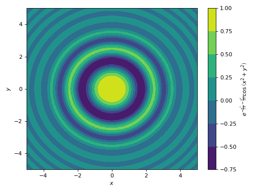
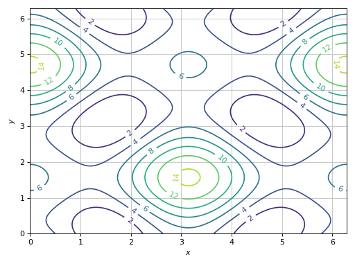
Line contours of a function of two variables, with ticks formatted as multiples of pi/n.
>>> expr = 5 * (cos(x) - 0.2 * sin(y))**2 + 5 * (-0.2 * cos(x) + sin(y))**2
>>> graphics(
...     contour(expr, (x, 0, 2 * pi), (y, 0, 2 * pi), fill=False),
...     x_ticks_formatter=multiples_of_pi_over_2(),
...     y_ticks_formatter=multiples_of_pi_over_3(),
...     aspect="equal"
... )
Plot object containing:
[0]: contour: 5*(-0.2*sin(y) + cos(x))**2 + 5*(sin(y) - 0.2*cos(x))**2 for x over (0, 2*pi) and y over (0, 2*pi)
(
Source code,png)
Combining together filled and line contours. Use a custom label on the colorbar of the filled contour.
>>> expr = 5 * (cos(x) - 0.2 * sin(y))**2 + 5 * (-0.2 * cos(x) + sin(y))**2
>>> graphics(
...     contour(expr, (x, 0, 2 * pi), (y, 0, 2 * pi), "z",
...         rendering_kw={"cmap": "coolwarm"}),
...     contour(expr, (x, 0, 2 * pi), (y, 0, 2 * pi),
...         rendering_kw={"colors": "k", "cmap": None, "linewidths": 0.75},
...         fill=False),
...     x_ticks_formatter=multiples_of_pi_over_2(),
...     y_ticks_formatter=multiples_of_pi_over_3(),
...     aspect="equal", grid=False
... )
Plot object containing:
[0]: contour: 5*(-0.2*sin(y) + cos(x))**2 + 5*(sin(y) - 0.2*cos(x))**2 for x over (0, 2*pi) and y over (0, 2*pi)
[1]: contour: 5*(-0.2*sin(y) + cos(x))**2 + 5*(sin(y) - 0.2*cos(x))**2 for x over (0, 2*pi) and y over (0, 2*pi)
(
Source code,png)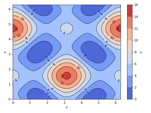
Visually inspect the solutions of a system of 2 non-linear equations. The intersections between the contour lines represent the solutions.
>>> eq1 = Eq((cos(x) - sin(y) / 2)**2 + 3 * (-sin(x) + cos(y) / 2)**2, 2)
>>> eq2 = Eq((cos(x) - 2 * sin(y))**2 - (sin(x) + 2 * cos(y))**2, 3)
>>> graphics(
...     contour(
...         eq1.lhs - eq1.rhs, (x, 0, 2 * pi), (y, 0, 2 * pi),
...         rendering_kw={"levels": [0]},
...         fill=False, clabels=False),
...     contour(
...         eq2.lhs - eq2.rhs, (x, 0, 2 * pi), (y, 0, 2 * pi),
...         rendering_kw={"levels": [0]},
...         fill=False, clabels=False),
... )
Plot object containing:
[0]: contour: 3*(-sin(x) + cos(y)/2)**2 + (-sin(y)/2 + cos(x))**2 - 2 for x over (0, 2*pi) and y over (0, 2*pi)
[1]: contour: -(sin(x) + 2*cos(y))**2 + (-2*sin(y) + cos(x))**2 - 3 for x over (0, 2*pi) and y over (0, 2*pi)
(
Source code,png)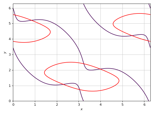
Contour plot with polar axis:
>>> r, theta = symbols("r, theta")
>>> graphics(
...     contour(
...         sin(2 * r) * cos(theta), (theta, 0, 2*pi), (r, 0, 7),
...         rendering_kw={"levels": 100}
...     ),
...     polar_axis=True, aspect="equal"
... )
Plot object containing:
[0]: contour: sin(2*r)*cos(theta) for theta over (0, 2*pi) and r over (0, 7)
(
Source code,png)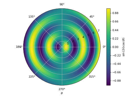
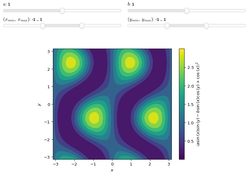
Interactive-widget plot. Refer to the interactive sub-module documentation to learn more about the
paramsdictionary. This plot illustrates:the use of
prange(parametric plotting range).the use of the
paramsdictionary to specify sliders in their basic form: (default, min, max).the use of
panel.widgets.slider.RangeSlider, which is a 2-values widget.
from sympy import *
from spb import *
import panel as pn
x, y, a, b = symbols("x y a b")
x_min, x_max, y_min, y_max = symbols("x_min x_max y_min y_max")
expr = (cos(x) + a * sin(x) * sin(y) - b * sin(x) * cos(y))**2
graphics(
    contour(
        expr, prange(x, x_min*pi, x_max*pi), prange(y, y_min*pi, y_max*pi),
        params={
            a: (1, 0, 2), b: (1, 0, 2),
            (x_min, x_max): pn.widgets.RangeSlider(
                value=(-1, 1), start=-3, end=3, step=0.1),
            (y_min, y_max): pn.widgets.RangeSlider(
                value=(-1, 1), start=-3, end=3, step=0.1),
        }),
    grid=False
)
- spb.graphics.functions_2d.implicit_2d(f, range_x=None, range_y=None, label=None, rendering_kw=None, color=None, border_color=None, border_kw=None, **kwargs)[source]
Plot implicit equations / inequalities.
implicit_2d, by default, generates a contour using a mesh grid of fixednumber of points. The greater the number of points, the better the results, but also the greater the memory used. By settingadaptive=True, interval arithmetic will be used to plot functions. If the expression cannot be plotted using interval arithmetic, it defaults to generating a contour using a mesh grid. With interval arithmetic, the line width can become very small; in those cases, it is better to use the mesh grid approach.- Parameters:
- fRelational, Boolean, Expr
The equation / inequality that is to be plotted.
- range_xtuple, Tuple
A 3-tuple (symb, min, max) denoting the range of the x variable. Default values: min=-10 and max=10.
- range_ytuple, Tuple
A 3-tuple (symb, min, max) denoting the range of the y variable. Default values: min=-10 and max=10.
- labelstr
Set the label associated to this series, which will be eventually shown on the legend or colorbar.
- rendering_kwdict
A dictionary of keyword arguments to be passed to the renderers in order to further customize the appearance of the contour. Here are some useful links for the supported plotting libraries:
- colorstr, optional
Specify the color of lines/regions. Default to None (automatic coloring by the backend).
- border_colorstr or bool, optional
If given, a limiting border will be added when plotting inequalities (<, <=, >, >=). Use
border_kwif more customization options are required.- border_kwdict, optional
If given, a limiting border will be added when plotting inequalities (<, <=, >, >=). This is a dictionary of keywords/values which is passed to the backend’s function to customize the appearance of the limiting border. Refer to the plotting library (backend) manual for more informations.
- adaptivebool
Select the evaluation strategy to be used. If
False, the internal algorithm uses a mesh grid approach. In such case, Boolean combinations of expressions cannot be plotted. IfTrue, the internal algorithm uses interval arithmetic. If the expression cannot be plotted with interval arithmetic, it switches to the meshgrid approach. Default value: False.- colorbarbool
Toggle the visibility of the colorbar associated to the current data series. Note that a colorbar is only visible if
use_cm=Trueandcolor_funcis not None. Default value: True.- depthint
The depth of recursion for adaptive grid. Think of the resulting plot as a picture composed by pixels. Increasing
depthwill increase the number of pixels, thus obtaining a more accurate plot, at the cost of evaluation speed and possibly readability (if the figure has small size). It must be: 0 ≤ depth ≤ 4. Default value: 0.- force_real_evalbool
By default, numerical evaluation is performed over complex numbers, which is slower but produces correct results. However, when the symbolic expression is converted to a numerical function with lambdify, the resulting function may not like to be evaluated over complex numbers. In such cases, forcing the evaluation to be performed over real numbers might be a good choice. The plotting module should be able to detect such occurences and automatically activate this option. If that is not the case, or evaluation performance is of paramount importance, set this parameter to True, but be aware that it might produce wrong results. Default value: False.
- modules
Specify the evaluation modules to be used by lambdify. If not specified, the evaluation will be done with NumPy/SciPy.
- n1int
Number of discretization points along the x-axis to be used in the evaluation, when
adaptive=False. Related parameters:adaptive, xscale. It must be: 2 ≤ n1 < ∞. Default value: 100.- n2int
Number of discretization points along the y-axis to be used in the evaluation, when
adaptive=False. Related parameters:adaptive, yscale. It must be: 2 ≤ n2 < ∞. Default value: 100.- only_integersbool
Discretize the domain using only integer numbers. When this parameter is True, the number of discretization points is choosen by the algorithm. Default value: False.
- paramsdict, optional
A dictionary mapping symbols to parameters. If provided, this dictionary enables the interactive-widgets plot.
When calling a plotting function, the parameter can be specified with:
a widget from the
ipywidgetsmodule.a widget from the
panelmodule.- a tuple of the form:
(default, min, max, N, tick_format, label, spacing), which will instantiate a
ipywidgets.widgets.widget_float.FloatSlideror aipywidgets.widgets.widget_float.FloatLogSlider, depending on the spacing strategy. In particular:- default, min, maxfloat
Default value, minimum value and maximum value of the slider, respectively. Must be finite numbers. The order of these 3 numbers is not important: the module will figure it out which is what.
- Nint, optional
Number of steps of the slider.
- tick_formatstr or None, optional
Provide a formatter for the tick value of the slider. Default to
".2f".
- label: str, optional
Custom text associated to the slider.
- spacingstr, optional
Specify the discretization spacing. Default to
"linear", can be changed to"log".
Notes:
parameters cannot be linked together (ie, one parameter cannot depend on another one).
If a widget returns multiple numerical values (like
panel.widgets.slider.RangeSlideroripywidgets.widgets.widget_float.FloatRangeSlider), then a corresponding number of symbols must be provided.
Here follows a couple of examples. If
imodule="panel":import panel as pn params = { a: (1, 0, 5), # slider from 0 to 5, with default value of 1 b: pn.widgets.FloatSlider(value=1, start=0, end=5), # same slider as above (c, d): pn.widgets.RangeSlider(value=(-1, 1), start=-3, end=3, step=0.1) }
Or with
imodule="ipywidgets":import ipywidgets as w params = { a: (1, 0, 5), # slider from 0 to 5, with default value of 1 b: w.FloatSlider(value=1, min=0, max=5), # same slider as above (c, d): w.FloatRangeSlider(value=(-1, 1), min=-3, max=3, step=0.1) }
When instantiating a data series directly,
paramsmust be a dictionary mapping symbols to numerical values.Let
seriesbe any data series. Thenseries.paramsreturns a dictionary mapping symbols to numerical values.- show_in_legendbool
Toggle the visibility of the data series on the legend. Default value: True.
- sum_boundint
When plotting sums, the expression will be pre-processed in order to replace lower/upper bounds set to +/- infinity with this +/- numerical value. Note: the higher this number, the slower the evaluation, but the more accurate the plot. It must be: 0 ≤ sum_bound < ∞. Default value: 1000.
- use_cmbool
Toggle the use of a colormap. By default, some series might use a colormap to display the necessary data. Setting this attribute to False will inform the associated renderer to use solid color. Related parameters:
color_func. Default value: False.- xscalestr
Discretization strategy along the x-direction. Related parameters:
n1. Possible options: [‘linear’, ‘log’] Default value: ‘linear’.- yscalestr
Discretization strategy along the y-direction. Related parameters:
n2. Possible options: [‘linear’, ‘log’] Default value: ‘linear’.
- Returns:
- serieslist
A list containing at most two instances of
Implicit2DSeries.
See also
Examples
Plot expressions:
>>> from sympy import symbols, Ne, Eq, And, sin, cos, pi, log, latex
>>> from spb import *
>>> x, y = symbols('x y')
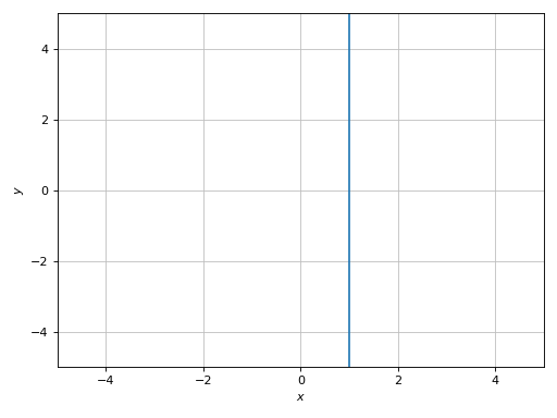
Plot a line representing an equality:
>>> graphics(implicit_2d(x - 1, (x, -5, 5), (y, -5, 5)))
Plot object containing:
[0]: Implicit expression: Eq(x - 1, 0) for x over (-5, 5) and y over (-5, 5)
(
Source code,png)
Plot a region:
>>> graphics(
...     implicit_2d(y > x**2, (x, -5, 5), (y, -10, 10), n=150),
...     grid=False)
Plot object containing:
[0]: Implicit expression: y > x**2 for x over (-5, 5) and y over (-10, 10)
(
Source code,png)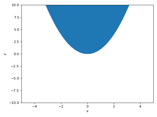
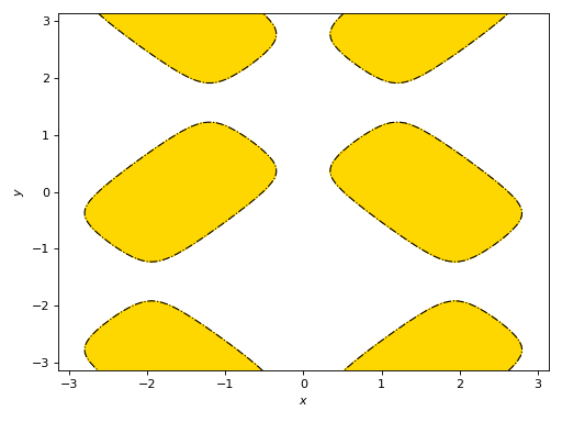
Plot a region using a custom color, highlights the limiting border and customize its appearance.
>>> expr = 4 * (cos(x) - sin(y) / 5)**2 + 4 * (-cos(x) / 5 + sin(y))**2
>>> graphics(
...     implicit_2d(
...         expr <= pi, (x, -pi, pi), (y, -pi, pi),
...         color="gold", border_color="k",
...         border_kw={"linestyles": "-.", "linewidths": 1}
...     ),
...     grid=False
... )
Plot object containing:
[0]: Implicit expression: 4*(-sin(y)/5 + cos(x))**2 + 4*(sin(y) - cos(x)/5)**2 <= pi for x over (-pi, pi) and y over (-pi, pi)
[1]: Implicit expression: Eq(-4*(-sin(y)/5 + cos(x))**2 - 4*(sin(y) - cos(x)/5)**2 + pi, 0) for x over (-pi, pi) and y over (-pi, pi)
(
Source code,png)
Boolean expressions will be plotted with the adaptive algorithm. Note the thin width of lines:
>>> graphics(
...     implicit_2d(
...         Eq(y, sin(x)) & (y > 0), (x, -2 * pi, 2 * pi), (y, -4, 4)),
...     implicit_2d(
...         Eq(y, sin(x)) & (y < 0), (x, -2 * pi, 2 * pi), (y, -4, 4)),
...     ylim=(-2, 2)
... )
Plot object containing:
[0]: Implicit expression: (y > 0) & Eq(y, sin(x)) for x over (-2*pi, 2*pi) and y over (-4, 4)
[1]: Implicit expression: (y < 0) & Eq(y, sin(x)) for x over (-2*pi, 2*pi) and y over (-4, 4)
(
Source code,png)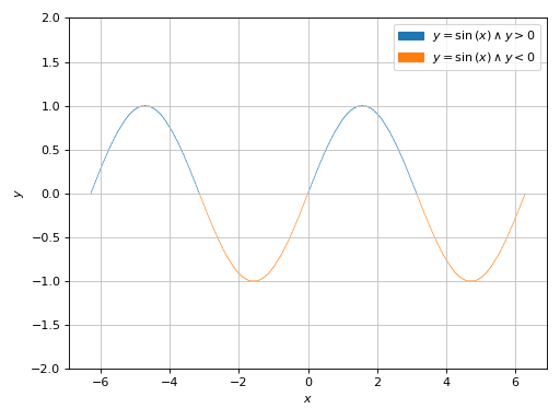
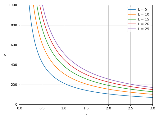
Plotting multiple implicit expressions and setting labels:
>>> V, t, b, L = symbols("V, t, b, L")
>>> L_array = [5, 10, 15, 20, 25]
>>> b_val = 0.0032
>>> expr = b * V * 0.277 * t - b * L - log(1 + b * V * 0.277 * t)
>>> series = []
>>> for L_val in L_array:
...     series += implicit_2d(
...         expr.subs({b: b_val, L: L_val}), (t, 0, 3), (V, 0, 1000),
...         label="L = %s" % L_val)
>>> graphics(*series)
Plot object containing:
[0]: Implicit expression: Eq(0.0008864*V*t - log(0.0008864*V*t + 1) - 0.016, 0) for t over (0, 3) and V over (0, 1000)
[1]: Implicit expression: Eq(0.0008864*V*t - log(0.0008864*V*t + 1) - 0.032, 0) for t over (0, 3) and V over (0, 1000)
[2]: Implicit expression: Eq(0.0008864*V*t - log(0.0008864*V*t + 1) - 0.048, 0) for t over (0, 3) and V over (0, 1000)
[3]: Implicit expression: Eq(0.0008864*V*t - log(0.0008864*V*t + 1) - 0.064, 0) for t over (0, 3) and V over (0, 1000)
[4]: Implicit expression: Eq(0.0008864*V*t - log(0.0008864*V*t + 1) - 0.08, 0) for t over (0, 3) and V over (0, 1000)
(
Source code,png)
Comparison of similar expressions plotted with different algorithms. Note:
Adaptive algorithm (
adaptive=True) can be used with any expression, but it usually creates lines with variable thickness. Thedepthkeyword argument can be used to improve the accuracy, but reduces line thickness even further.Mesh grid algorithm (
adaptive=False) creates lines with constant thickness.
>>> expr1 = Eq(x * y - 20, 15 * y)
>>> expr2 = Eq((x - 3) * y - 20, 15 * y)
>>> expr3 = Eq((x - 6) * y - 20, 15 * y)
>>> ranges = (x, 15, 30), (y, 0, 50)
>>> graphics(
...    implicit_2d(
...        expr1, *ranges, adaptive=True, depth=0,
...        label="adaptive=True, depth=0"),
...    implicit_2d(
...        expr2, *ranges, adaptive=True, depth=1,
...        label="adaptive=True, depth=1"),
...    implicit_2d(
...        expr3, *ranges, adaptive=False, label="adaptive=False"),
...    grid=False
... )
Plot object containing:
[0]: Implicit expression: Eq(x*y - 20, 15*y) for x over (15, 30) and y over (0, 50)
[1]: Implicit expression: Eq(y*(x - 3) - 20, 15*y) for x over (15, 30) and y over (0, 50)
[2]: Implicit expression: Eq(y*(x - 6) - 20, 15*y) for x over (15, 30) and y over (0, 50)
(
Source code,png)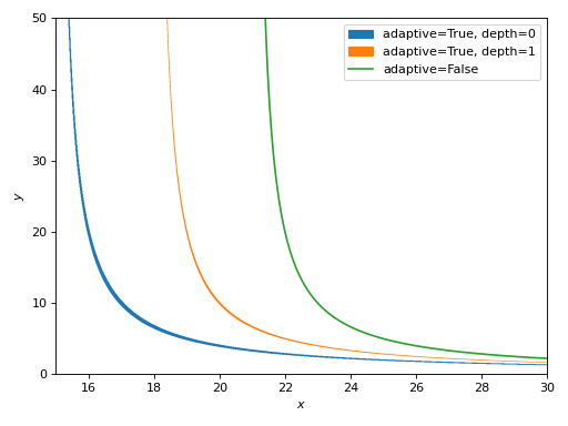
If the expression is plotted with the adaptive algorithm and it produces “low-quality” results, maybe it’s possible to rewrite it in order to use the mesh grid approach (contours). For example:
>>> from spb import plotgrid
>>> expr = Ne(x*y, 1)
>>> p1 = graphics(
...     implicit_2d(expr, (x, -10, 10), (y, -10, 10)),
...     grid=False, title="$%s$ : First approach" % latex(expr),
...     aspect="equal", show=False)
>>> p2 = graphics(
...     implicit_2d(x < 20, (x, -10, 10), (y, -10, 10)),
...     implicit_2d(Eq(*expr.args), (x, -10, 10), (y, -10, 10),
...         color="w", show_in_legend=False),
...     grid=False, title="$%s$ : Second approach" % latex(expr),
...     aspect="equal", show=False)
>>> plotgrid(p1, p2, nc=2)
(
Source code,png)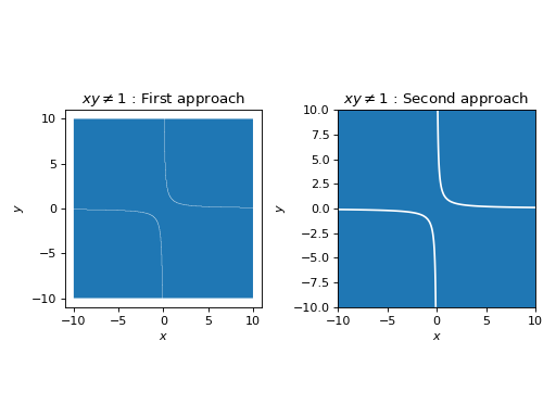
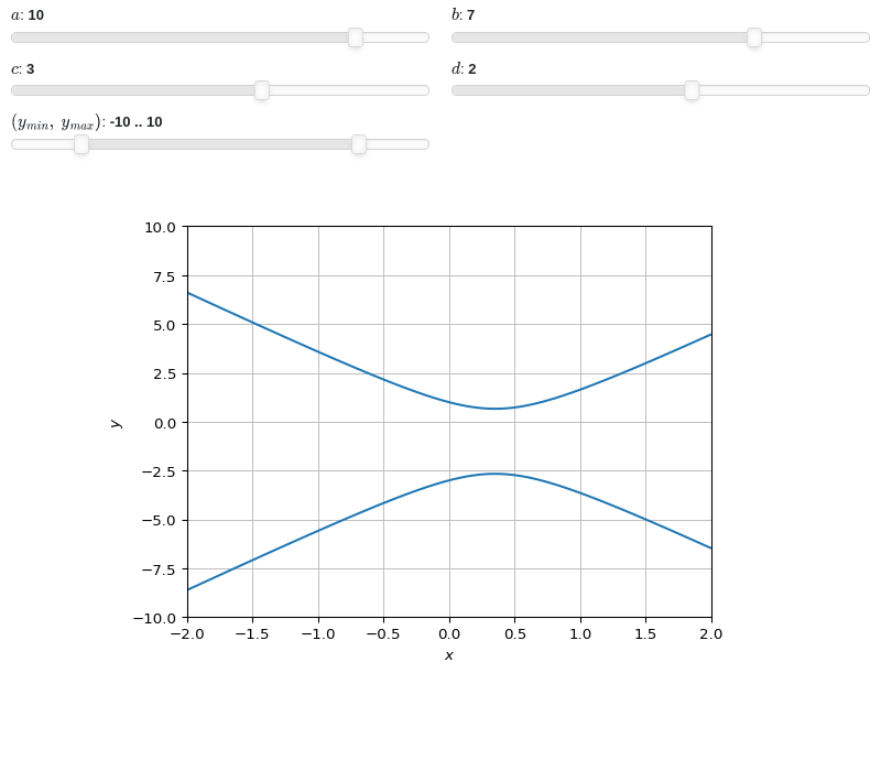
Interactive-widget implicit plot. Refer to the interactive sub-module documentation to learn more about the
paramsdictionary. This plot illustrates:the use of
prange(parametric plotting range).the use of the
paramsdictionary to specify sliders in their basic form: (default, min, max).the use of
panel.widgets.slider.RangeSlider, which is a 2-values widget.
from sympy import *
from spb import *
import panel as pn
x, y, a, b, c, d = symbols("x, y, a, b, c, d")
y_min, y_max = symbols("y_min, y_max")
expr = Eq(a * x**2 - b * x + c, d * y + y**2)
graphics(
    implicit_2d(expr, (x, -2, 2), prange(y, y_min, y_max),
        params={
            a: (10, -15, 15),
            b: (7, -15, 15),
            c: (3, -15, 15),
            d: (2, -15, 15),
            (y_min, y_max): pn.widgets.RangeSlider(
                value=(-10, 10), start=-15, end=15, step=0.1)
        }, n=150),
    ylim=(-10, 10))
- spb.graphics.functions_2d.list_2d(list_x, list_y, label=None, rendering_kw=None, **kwargs)[source]
Plots lists of coordinates.
- Parameters:
- list_x
Coordinates for the x-axis. It can be a list or a numper array.
- list_y
Coordinates for the y-axis. It can be a list or a numper array.
- labelstr
Set the label associated to this series, which will be eventually shown on the legend or colorbar.
- rendering_kwdict
A dictionary of keyword arguments to be passed to the renderers in order to further customize the appearance of the line. Here are some useful links for the supported plotting libraries:
Matplotlib:
for solid lines: https://matplotlib.org/stable/api/_as_gen/matplotlib.pyplot.plot.html
for colormap-based lines: https://matplotlib.org/stable/api/collections_api.html#matplotlib.collections.LineCollection
for scatters: https://matplotlib.org/stable/api/_as_gen/matplotlib.pyplot.scatter.html
Bokeh:
- color_funccallable
A color function to be applied to the numerical data. It can be:
None: no color function.
callable: a function accepting:
no arguments: this can be used to return an array of precomputed values.
two arguments, the x, y coordinates.
- colorbarbool
Toggle the visibility of the colorbar associated to the current data series. Note that a colorbar is only visible if
use_cm=Trueandcolor_funcis not None. Default value: True.- colorbar_ticks_formattertick_formatter_multiples_of
An object of type
tick_formatter_multiples_ofwhich will be used to place tick values on the colorbar at each multiple of a specified quantity. This only works when use_cm=True.- is_filledbool
Whether scatter’s markers are filled or void. Default value: True.
- is_scatterbool
If True it represent a scatter plot, otherwise a continuous line. Default value: False.
- line_color
For back-compatibility with old sympy.plotting. Use
rendering_kwin order to fully customize the appearance of the line/scatter.- paramsdict, optional
A dictionary mapping symbols to parameters. If provided, this dictionary enables the interactive-widgets plot.
When calling a plotting function, the parameter can be specified with:
a widget from the
ipywidgetsmodule.a widget from the
panelmodule.- a tuple of the form:
(default, min, max, N, tick_format, label, spacing), which will instantiate a
ipywidgets.widgets.widget_float.FloatSlideror aipywidgets.widgets.widget_float.FloatLogSlider, depending on the spacing strategy. In particular:- default, min, maxfloat
Default value, minimum value and maximum value of the slider, respectively. Must be finite numbers. The order of these 3 numbers is not important: the module will figure it out which is what.
- Nint, optional
Number of steps of the slider.
- tick_formatstr or None, optional
Provide a formatter for the tick value of the slider. Default to
".2f".
- label: str, optional
Custom text associated to the slider.
- spacingstr, optional
Specify the discretization spacing. Default to
"linear", can be changed to"log".
Notes:
parameters cannot be linked together (ie, one parameter cannot depend on another one).
If a widget returns multiple numerical values (like
panel.widgets.slider.RangeSlideroripywidgets.widgets.widget_float.FloatRangeSlider), then a corresponding number of symbols must be provided.
Here follows a couple of examples. If
imodule="panel":import panel as pn params = { a: (1, 0, 5), # slider from 0 to 5, with default value of 1 b: pn.widgets.FloatSlider(value=1, start=0, end=5), # same slider as above (c, d): pn.widgets.RangeSlider(value=(-1, 1), start=-3, end=3, step=0.1) }
Or with
imodule="ipywidgets":import ipywidgets as w params = { a: (1, 0, 5), # slider from 0 to 5, with default value of 1 b: w.FloatSlider(value=1, min=0, max=5), # same slider as above (c, d): w.FloatRangeSlider(value=(-1, 1), min=-3, max=3, step=0.1) }
When instantiating a data series directly,
paramsmust be a dictionary mapping symbols to numerical values.Let
seriesbe any data series. Thenseries.paramsreturns a dictionary mapping symbols to numerical values.- show_in_legendbool
Toggle the visibility of the data series on the legend. Default value: True.
- stepsNoneType, bool, str
If set, it connects consecutive points with steps rather than straight segments. Possible options: [‘pre’, ‘post’, ‘mid’, True, False, None] Default value: False.
- txcallable
Numerical transformation function to be applied to the data on the x-axis.
- tycallable
Numerical transformation function to be applied to the data on the y-axis.
- unwrapbool, dict
Whether to use numpy.unwrap() on the computed coordinates in order to get rid of discontinuities. It can be:
False: do not use
np.unwrap().True: use
np.unwrap()with default keyword arguments.dictionary of keyword arguments passed to
np.unwrap().
- use_cmbool
Toggle the use of a colormap. By default, some series might use a colormap to display the necessary data. Setting this attribute to False will inform the associated renderer to use solid color. Related parameters:
color_func. Default value: False.
- Returns:
- serieslist
A list containing one instance of
List2DSeries.
See also
Examples
>>> from sympy import symbols, sin, cos
>>> from spb import *
>>> x = symbols('x')
Plot the coordinates of a single function:
>>> xx = [t / 100 * 6 - 3 for t in list(range(101))]
>>> yy = [cos(x).evalf(subs={x: t}) for t in xx]
>>> graphics(list_2d(xx, yy))
Plot object containing:
[0]: 2D list plot
(
Source code,png)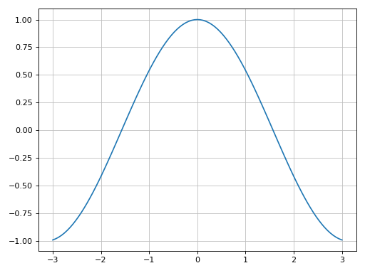
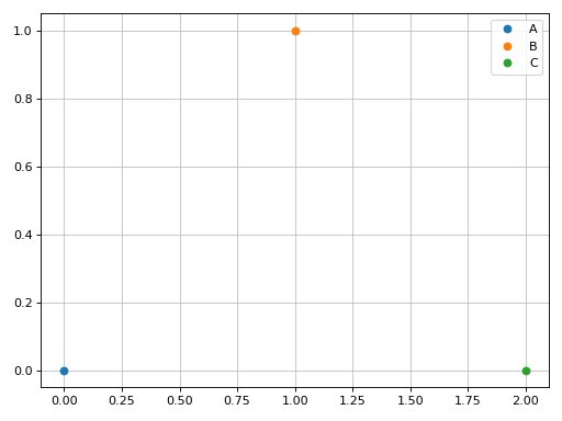
Plot individual points with custom labels. Each point will be converted to a list by the algorithm:
>>> graphics(
...     list_2d(0, 0, "A", is_scatter=True),
...     list_2d(1, 1, "B", is_scatter=True),
...     list_2d(2, 0, "C", is_scatter=True),
... )
Plot object containing:
[0]: 2D list plot
[1]: 2D list plot
[2]: 2D list plot
(
Source code,png)
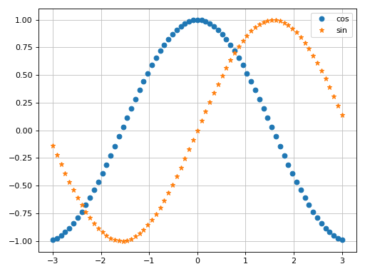
Scatter plot of the coordinates of multiple functions, with custom rendering keywords:
>>> xx = [t / 70 * 6 - 3 for t in list(range(71))]
>>> yy1 = [cos(x).evalf(subs={x: t}) for t in xx]
>>> yy2 = [sin(x).evalf(subs={x: t}) for t in xx]
>>> graphics(
...     list_2d(xx, yy1, "cos", is_scatter=True),
...     list_2d(xx, yy2, "sin", {"marker": "*", "markerfacecolor": None},
...             is_scatter=True),
... )
Plot object containing:
[0]: 2D list plot
[1]: 2D list plot
(
Source code,png)
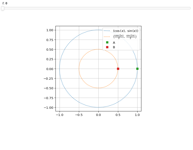
Interactive-widget plot. Refer to the interactive sub-module documentation to learn more about the
paramsdictionary.from sympy import * from spb import * x, t = symbols("x, t") params = {t: (0, 0, 2*pi)} graphics( line_parametric_2d( cos(x), sin(x), (x, 0, 2*pi), rendering_kw={"linestyle": ":"}, use_cm=False), line_parametric_2d( cos(2 * x) / 2, sin(2 * x) / 2, (x, 0, pi), rendering_kw={"linestyle": ":"}, use_cm=False), list_2d( cos(t), sin(t), "A", rendering_kw={"marker": "s", "markerfacecolor": None}, params=params, is_scatter=True), list_2d( cos(2 * t) / 2, sin(2 * t) / 2, "B", rendering_kw={"marker": "s", "markerfacecolor": None}, params=params, is_scatter=True), aspect="equal" )
- spb.graphics.functions_2d.geometry(geom, label=None, rendering_kw=None, fill=True, **kwargs)[source]
Plot entities from the sympy.geometry module.
- Parameters:
- geomGeometryEntity
Represent the geometric entity to be plotted.
- labelstr
Set the label associated to this series, which will be eventually shown on the legend or colorbar.
- rendering_kwdict
A dictionary of keyword arguments to be passed to the renderers in order to further customize the appearance of the line. Here are some useful links for the supported plotting libraries:
Matplotlib:
for solid lines: https://matplotlib.org/stable/api/_as_gen/matplotlib.pyplot.plot.html
for colormap-based lines: https://matplotlib.org/stable/api/collections_api.html#matplotlib.collections.LineCollection
for scatters: https://matplotlib.org/stable/api/_as_gen/matplotlib.pyplot.scatter.html
Bokeh:
- colorbar_ticks_formattertick_formatter_multiples_of
An object of type
tick_formatter_multiples_ofwhich will be used to place tick values on the colorbar at each multiple of a specified quantity. This only works when use_cm=True.- is_filledbool
If True, the geometry will be filled, otherwise only the perimeter will be rendered. Default value: True.
- is_scatterbool
If True it represent a scatter plot, otherwise a continuous line. Default value: False.
- line_color
For back-compatibility with old sympy.plotting. Use
rendering_kwin order to fully customize the appearance of the line/scatter.- n1int
Number of discretization points used to resolve the polar angle theta ∈ [0, 2*pi] in order to plot ellipses. It must be: 2 ≤ n1 < ∞. Default value: 1000.
- paramsdict, optional
A dictionary mapping symbols to parameters. If provided, this dictionary enables the interactive-widgets plot.
When calling a plotting function, the parameter can be specified with:
a widget from the
ipywidgetsmodule.a widget from the
panelmodule.- a tuple of the form:
(default, min, max, N, tick_format, label, spacing), which will instantiate a
ipywidgets.widgets.widget_float.FloatSlideror aipywidgets.widgets.widget_float.FloatLogSlider, depending on the spacing strategy. In particular:- default, min, maxfloat
Default value, minimum value and maximum value of the slider, respectively. Must be finite numbers. The order of these 3 numbers is not important: the module will figure it out which is what.
- Nint, optional
Number of steps of the slider.
- tick_formatstr or None, optional
Provide a formatter for the tick value of the slider. Default to
".2f".
- label: str, optional
Custom text associated to the slider.
- spacingstr, optional
Specify the discretization spacing. Default to
"linear", can be changed to"log".
Notes:
parameters cannot be linked together (ie, one parameter cannot depend on another one).
If a widget returns multiple numerical values (like
panel.widgets.slider.RangeSlideroripywidgets.widgets.widget_float.FloatRangeSlider), then a corresponding number of symbols must be provided.
Here follows a couple of examples. If
imodule="panel":import panel as pn params = { a: (1, 0, 5), # slider from 0 to 5, with default value of 1 b: pn.widgets.FloatSlider(value=1, start=0, end=5), # same slider as above (c, d): pn.widgets.RangeSlider(value=(-1, 1), start=-3, end=3, step=0.1) }
Or with
imodule="ipywidgets":import ipywidgets as w params = { a: (1, 0, 5), # slider from 0 to 5, with default value of 1 b: w.FloatSlider(value=1, min=0, max=5), # same slider as above (c, d): w.FloatRangeSlider(value=(-1, 1), min=-3, max=3, step=0.1) }
When instantiating a data series directly,
paramsmust be a dictionary mapping symbols to numerical values.Let
seriesbe any data series. Thenseries.paramsreturns a dictionary mapping symbols to numerical values.- range_xtuple
A 2-tuple (min, max) denoting the range of the x variable to be used when plotting objects of type Line2D. If not provided, a segment will be plotted between the 2 specified points of the line.
- show_in_legendbool
Toggle the visibility of the data series on the legend. Default value: True.
- txcallable
Numerical transformation function to be applied to the data on the x-axis.
- tycallable
Numerical transformation function to be applied to the data on the y-axis.
- Returns:
- serieslist
A list containing one instance of
GeometrySeries.
See also
Examples
>>> from sympy import (symbols, Circle, Ellipse, Polygon,
...      Curve, Segment, Point2D, Point3D, Line3D, Plane,
...      Rational, pi, Point, cos, sin)
>>> from spb import *
>>> x, y, z = symbols('x, y, z')
Plot a single geometry, customizing its color:
>>> graphics(
...     geometry(
...         Ellipse(Point(-3, 2), hradius=3, eccentricity=Rational(4, 5)),
...         rendering_kw={"color": "tab:orange"}),
...     grid=False, aspect="equal"
... )
Plot object containing:
[0]: 2D geometry entity: Ellipse(Point2D(-3, 2), 3, 9/5)
(
Source code,png)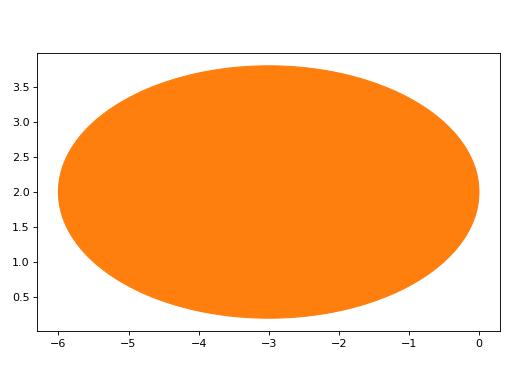
Plot several numeric geometric entitiesy. By default, circles, ellipses and polygons are going to be filled. Plotting Curve objects is the same as plot_parametric.
>>> graphics(
...     geometry(Circle(Point(0, 0), 5)),
...     geometry(Ellipse(Point(-3, 2), hradius=3, eccentricity=Rational(4, 5))),
...     geometry(Polygon((4, 0), 4, n=5)),
...     geometry(Curve((cos(x), sin(x)), (x, 0, 2 * pi))),
...     geometry(Segment((-4, -6), (6, 6))),
...     geometry(Point2D(0, 0)),
...     aspect="equal", grid=False
... )
Plot object containing:
[0]: 2D geometry entity: Circle(Point2D(0, 0), 5)
[1]: 2D geometry entity: Ellipse(Point2D(-3, 2), 3, 9/5)
[2]: 2D geometry entity: RegularPolygon(Point2D(4, 0), 4, 5, 0)
[3]: parametric cartesian line: (cos(x), sin(x)) for x over (0, 2*pi)
[4]: 2D geometry entity: Segment2D(Point2D(-4, -6), Point2D(6, 6))
[5]: 2D geometry entity: Point2D(0, 0)
(
Source code,png)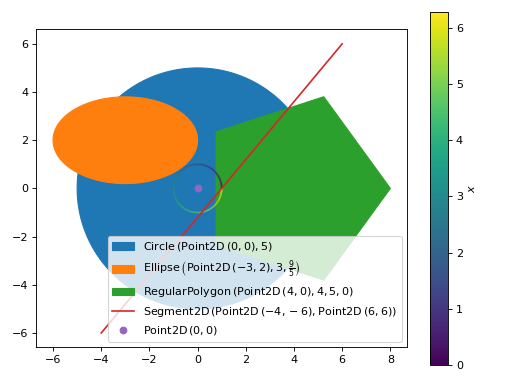
Plot several numeric geometric entities defined by numbers only, turn off fill. Every entity is represented as a line.
>>> graphics(
...     geometry(Circle(Point(0, 0), 5), fill=False),
...     geometry(
...         Ellipse(Point(-3, 2), hradius=3, eccentricity=Rational(4, 5)),
...         fill=False),
...     geometry(Polygon((4, 0), 4, n=5), fill=False),
...     geometry(Curve((cos(x), sin(x)), (x, 0, 2 * pi)), fill=False),
...     geometry(Segment((-4, -6), (6, 6)), fill=False),
...     geometry(Point2D(0, 0), fill=False),
...     aspect="equal", grid=False
... )
Plot object containing:
[0]: 2D geometry entity: Circle(Point2D(0, 0), 5)
[1]: 2D geometry entity: Ellipse(Point2D(-3, 2), 3, 9/5)
[2]: 2D geometry entity: RegularPolygon(Point2D(4, 0), 4, 5, 0)
[3]: parametric cartesian line: (cos(x), sin(x)) for x over (0, 2*pi)
[4]: 2D geometry entity: Segment2D(Point2D(-4, -6), Point2D(6, 6))
[5]: 2D geometry entity: Point2D(0, 0)
(
Source code,png)
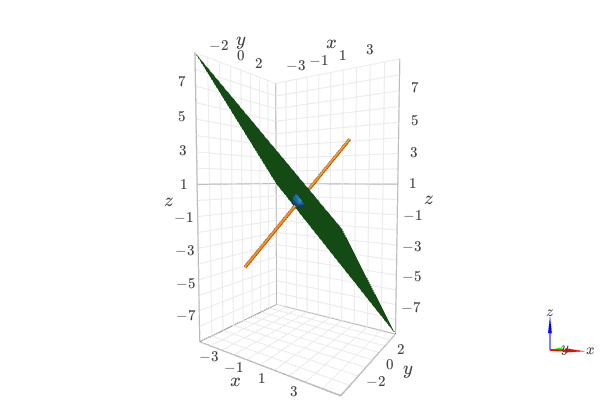
Plot 3D geometric entities. Instances of
Planemust be plotted withimplicit_3dor withplane(with the necessary ranges).from sympy import * from spb import * x, y, z = symbols("x, y, z") graphics( geometry( Point3D(0, 0, 0), label="center", rendering_kw={"point_size": 1}), geometry(Line3D(Point3D(-2, -3, -4), Point3D(2, 3, 4)), "line"), plane( Plane((0, 0, 0), (1, 1, 1)), (x, -5, 5), (y, -4, 4), (z, -10, 10)), backend=KB )
Interactive-widget plot. Refer to the interactive sub-module documentation to learn more about the
paramsdictionary.from sympy import * from spb import * import panel as pn a, b, c, d = symbols("a, b, c, d") params = { a: (0, -1, 1), b: (1, -1, 1), c: (2, 1, 2), d: pn.widgets.IntInput(value=6, start=3, end=8, name="n") } graphics( geometry(Polygon((a, b), c, n=d), "a", params=params), geometry( Polygon((a + 2, b + 3), c, n=d + 1), "b", params=params, fill=False), aspect="equal", xlim=(-2.5, 5.5), ylim=(-3, 6.5), imodule="panel")

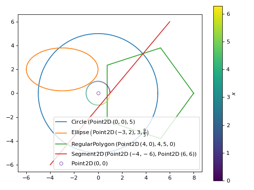
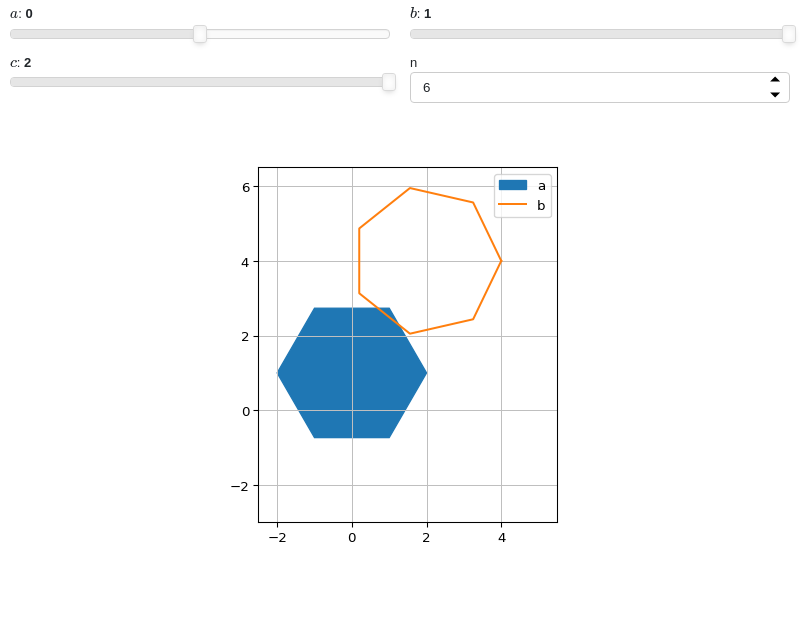
- spb.graphics.functions_2d.hline(y, label=None, rendering_kw=None, show_in_legend=True, **kwargs)[source]
Create an horizontal line at a given location in a 2D space.
- Parameters:
- yExpr
The y-coordinate where to draw the horizontal line.
- labelstr
Set the label associated to this series, which will be eventually shown on the legend or colorbar.
- rendering_kwdict
Keyword arguments to be passed to the renderers of the selected plotting library in order to further customize the appearance of this data series.
- show_in_legendbool
Toggle the visibility of the data series on the legend. Default value: True.
- paramsdict, optional
A dictionary mapping symbols to parameters. If provided, this dictionary enables the interactive-widgets plot.
When calling a plotting function, the parameter can be specified with:
a widget from the
ipywidgetsmodule.a widget from the
panelmodule.- a tuple of the form:
(default, min, max, N, tick_format, label, spacing), which will instantiate a
ipywidgets.widgets.widget_float.FloatSlideror aipywidgets.widgets.widget_float.FloatLogSlider, depending on the spacing strategy. In particular:- default, min, maxfloat
Default value, minimum value and maximum value of the slider, respectively. Must be finite numbers. The order of these 3 numbers is not important: the module will figure it out which is what.
- Nint, optional
Number of steps of the slider.
- tick_formatstr or None, optional
Provide a formatter for the tick value of the slider. Default to
".2f".
- label: str, optional
Custom text associated to the slider.
- spacingstr, optional
Specify the discretization spacing. Default to
"linear", can be changed to"log".
Notes:
parameters cannot be linked together (ie, one parameter cannot depend on another one).
If a widget returns multiple numerical values (like
panel.widgets.slider.RangeSlideroripywidgets.widgets.widget_float.FloatRangeSlider), then a corresponding number of symbols must be provided.
Here follows a couple of examples. If
imodule="panel":import panel as pn params = { a: (1, 0, 5), # slider from 0 to 5, with default value of 1 b: pn.widgets.FloatSlider(value=1, start=0, end=5), # same slider as above (c, d): pn.widgets.RangeSlider(value=(-1, 1), start=-3, end=3, step=0.1) }
Or with
imodule="ipywidgets":import ipywidgets as w params = { a: (1, 0, 5), # slider from 0 to 5, with default value of 1 b: w.FloatSlider(value=1, min=0, max=5), # same slider as above (c, d): w.FloatRangeSlider(value=(-1, 1), min=-3, max=3, step=0.1) }
When instantiating a data series directly,
paramsmust be a dictionary mapping symbols to numerical values.Let
seriesbe any data series. Thenseries.paramsreturns a dictionary mapping symbols to numerical values.
- Returns:
- A list containing one instance of
HVLineSeries.
- A list containing one instance of
See also
Examples
>>> from sympy import *
>>> from spb import *
>>> x = symbols("x")
>>> graphics(
...     line(cos(x), (x, -pi, pi)),
...     hline(
...         0.5, rendering_kw={"linestyle": ":"},
...         show_in_legend=False),
...     grid=False
... )
Plot object containing:
[0]: cartesian line: cos(x) for x over (-pi, pi)
[1]: horizontal line at y = 0.500000000000000
(
Source code,png)
Interactive widget plot:
from sympy import *
from spb import *
x, u, v, w = symbols("x u v w")
params = {
    u: (1, 0, 2),
    v: (1, 0, 2),
    w: (0.5, -1, 1)
}
graphics(
    line(u * cos(v * x), (x, -pi, pi), params=params),
    hline(
        w, rendering_kw={"linestyle": ":"},
        show_in_legend=False, params=params),
    grid=False, ylim=(-2, 2)
)
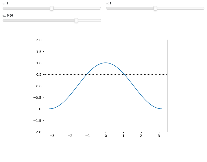
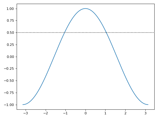
- spb.graphics.functions_2d.vline(x, label=None, rendering_kw=None, show_in_legend=True, **kwargs)[source]
Create an vertical line at a given location in a 2D space.
- Parameters:
- xExpr
The x-coordinate where to draw the vertical line.
- labelstr
Set the label associated to this series, which will be eventually shown on the legend or colorbar.
- rendering_kwdict
Keyword arguments to be passed to the renderers of the selected plotting library in order to further customize the appearance of this data series.
- show_in_legendbool
Toggle the visibility of the data series on the legend. Default value: True.
- paramsdict, optional
A dictionary mapping symbols to parameters. If provided, this dictionary enables the interactive-widgets plot.
When calling a plotting function, the parameter can be specified with:
a widget from the
ipywidgetsmodule.a widget from the
panelmodule.- a tuple of the form:
(default, min, max, N, tick_format, label, spacing), which will instantiate a
ipywidgets.widgets.widget_float.FloatSlideror aipywidgets.widgets.widget_float.FloatLogSlider, depending on the spacing strategy. In particular:- default, min, maxfloat
Default value, minimum value and maximum value of the slider, respectively. Must be finite numbers. The order of these 3 numbers is not important: the module will figure it out which is what.
- Nint, optional
Number of steps of the slider.
- tick_formatstr or None, optional
Provide a formatter for the tick value of the slider. Default to
".2f".
- label: str, optional
Custom text associated to the slider.
- spacingstr, optional
Specify the discretization spacing. Default to
"linear", can be changed to"log".
Notes:
parameters cannot be linked together (ie, one parameter cannot depend on another one).
If a widget returns multiple numerical values (like
panel.widgets.slider.RangeSlideroripywidgets.widgets.widget_float.FloatRangeSlider), then a corresponding number of symbols must be provided.
Here follows a couple of examples. If
imodule="panel":import panel as pn params = { a: (1, 0, 5), # slider from 0 to 5, with default value of 1 b: pn.widgets.FloatSlider(value=1, start=0, end=5), # same slider as above (c, d): pn.widgets.RangeSlider(value=(-1, 1), start=-3, end=3, step=0.1) }
Or with
imodule="ipywidgets":import ipywidgets as w params = { a: (1, 0, 5), # slider from 0 to 5, with default value of 1 b: w.FloatSlider(value=1, min=0, max=5), # same slider as above (c, d): w.FloatRangeSlider(value=(-1, 1), min=-3, max=3, step=0.1) }
When instantiating a data series directly,
paramsmust be a dictionary mapping symbols to numerical values.Let
seriesbe any data series. Thenseries.paramsreturns a dictionary mapping symbols to numerical values.
- Returns:
- A list containing one instance of
HVLineSeries.
- A list containing one instance of
See also
Examples
>>> from sympy import *
>>> from spb import *
>>> x = symbols("x")
>>> graphics(
...     line(cos(x), (x, -pi, pi)),
...     vline(1, rendering_kw={"linestyle": ":"}, show_in_legend=False),
...     vline(-1, rendering_kw={"linestyle": ":"}, show_in_legend=False),
...     grid=False
... )
Plot object containing:
[0]: cartesian line: cos(x) for x over (-pi, pi)
[1]: vertical line at x = 1
[2]: vertical line at x = -1
(
Source code,png)
Interactive widget plot:
from sympy import *
from spb import *
x, u, v, w = symbols("x u v w")
params = {
    u: (1, 0, 2),
    v: (1, 0, 2),
    w: (1, -pi, pi)
}
graphics(
    line(u * cos(v * x), (x, -pi, pi), params=params),
    vline(
        w, rendering_kw={"linestyle": ":"},
        show_in_legend=False, params=params),
    grid=False, ylim=(-2, 2)
)

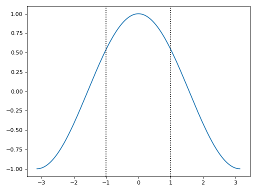
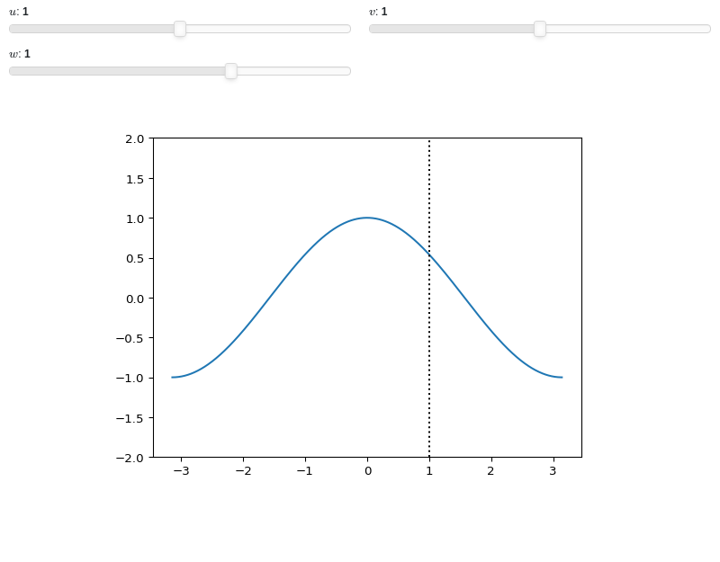