3D general plotting
NOTE:
For technical reasons, all interactive-widgets plots in this documentation
are created using Holoviz’s Panel. Often, they will ran just fine with
ipywidgets too. However, if a specific example uses the param library,
or widgets from the panel module, then users will have to modify the
params dictionary in order to make it work with ipywidgets.
Refer to Interactive module for more information.
- spb.graphics.functions_3d.line_parametric_3d(expr_x, expr_y, expr_z, range_p=None, label=None, rendering_kw=None, colorbar=True, use_cm=True, **kwargs)[source]
Plots a 3D parametric curve.
- Parameters:
- expr_x
The expression representing the component along the x-axis of the parametric function. It can either be a symbolic expression representing the function of one variable to be plotted, or a numerical function of one variable, supporting vectorization. In the latter case the following keyword arguments are not supported:
params,sum_bound.- expr_y
The expression representing the component along the y-axis of the parametric function. It can either be a symbolic expression representing the function of one variable to be plotted, or a numerical function of one variable, supporting vectorization. In the latter case the following keyword arguments are not supported:
params,sum_bound.- expr_z
The expression representing the component along the z-axis of the parametric function. It can either be a symbolic expression representing the function of one variable to be plotted, or a numerical function of one variable, supporting vectorization. In the latter case the following keyword arguments are not supported:
params,sum_bound.- range_ptuple, Tuple
A 3-tuple (symb, min, max) denoting the range of the parameter. Default values: min=-10 and max=10.
- labelstr
Set the label associated to this series, which will be eventually shown on the legend or colorbar.
- rendering_kwdict
A dictionary of keyword arguments to be passed to the renderers in order to further customize the appearance of the line. Here are some useful links for the supported plotting libraries:
Matplotlib:
for solid lines: https://matplotlib.org/stable/api/_as_gen/matplotlib.pyplot.plot.html
for colormap-based lines: https://matplotlib.org/stable/api/collections_api.html#matplotlib.collections.LineCollection
for scatters: https://matplotlib.org/stable/api/_as_gen/matplotlib.pyplot.scatter.html
Bokeh:
- colorbarbool
Toggle the visibility of the colorbar associated to the current data series. Note that a colorbar is only visible if
use_cm=Trueandcolor_funcis not None. Default value: True.- use_cmbool
Toggle the use of a colormap. By default, some series might use a colormap to display the necessary data. Setting this attribute to False will inform the associated renderer to use solid color. Related parameters:
color_func. Default value: False.- color_func
Define a custom color mapping when
use_cm=True. It can either be:A numerical function supporting vectorization. The arity can be:
1 argument:
f(t), wheretis the parameter.3 arguments:
f(x, y, z)wherex, y, zare the coordinates of the points.4 arguments:
f(x, y, z, t).
A symbolic expression having at most as many free symbols as
expr_xorexpr_yorexpr_z.None: the default value (color mapping according to the parameter).
Alias of this parameters:
tp.- colorbar_ticks_formattertick_formatter_multiples_of
An object of type
tick_formatter_multiples_ofwhich will be used to place tick values on the colorbar at each multiple of a specified quantity. This only works when use_cm=True.- detect_polesbool, str
Chose whether to detect and correctly plot the roots of the denominator. There are two algorithms at work:
based on the gradient of the numerical data, it introduces NaN values at locations where the steepness is greater than some threshold. This splits the line into multiple segments. To improve detection, increase the number of discretization points
nand/or change the value ofeps. This algorithm can be used to visualize jump discontinuities as well as essential discontinuities.a symbolic approach based on the
continuous_domainfunction from thesympy.calculus.utilmodule, which computes the locations of essential discontinuities. If any are found, vertical lines will be shown.
Possible options:
False: No poles detection
True: Poles detection with the numerical algorithm
‘symbolic’: Poles detection with numerical and symbolic algorithms
Default value: False.
- epsfloat
An arbitrary small value used by the
detect_polesnumerical algorithm. Before changing this value, it is recommended to increase the number of discretization points. Related parameters:detect_poles. It must be: 0 ≤ eps < ∞. Default value: 0.01.- excludelist
A list of numerical values along the parameter which are going to be excluded from the evaluation. In practice, it introduces discontinuities in the resulting line.
- force_real_evalbool
By default, numerical evaluation is performed over complex numbers, which is slower but produces correct results. However, when the symbolic expression is converted to a numerical function with lambdify, the resulting function may not like to be evaluated over complex numbers. In such cases, forcing the evaluation to be performed over real numbers might be a good choice. The plotting module should be able to detect such occurences and automatically activate this option. If that is not the case, or evaluation performance is of paramount importance, set this parameter to True, but be aware that it might produce wrong results. Default value: False.
- is_filledbool
Whether scatter’s markers are filled or void. Default value: True.
- is_scatterbool
If True it represent a scatter plot, otherwise a continuous line. Default value: False.
- line_color
For back-compatibility with old sympy.plotting. Use
rendering_kwin order to fully customize the appearance of the line/scatter.- modules
Specify the evaluation modules to be used by lambdify. If not specified, the evaluation will be done with NumPy/SciPy.
- n1int
Number of discretization points along the parameter to be used in the evaluation. An alias of this parameter is
n. Related parameters:xscale. It must be: 2 ≤ n1 < ∞. Default value: 1000.- only_integersbool
Discretize the domain using only integer numbers. When this parameter is True, the number of discretization points is choosen by the algorithm. Default value: False.
- paramsdict, optional
A dictionary mapping symbols to parameters. If provided, this dictionary enables the interactive-widgets plot.
When calling a plotting function, the parameter can be specified with:
a widget from the
ipywidgetsmodule.a widget from the
panelmodule.- a tuple of the form:
(default, min, max, N, tick_format, label, spacing), which will instantiate a
ipywidgets.widgets.widget_float.FloatSlideror aipywidgets.widgets.widget_float.FloatLogSlider, depending on the spacing strategy. In particular:- default, min, maxfloat
Default value, minimum value and maximum value of the slider, respectively. Must be finite numbers. The order of these 3 numbers is not important: the module will figure it out which is what.
- Nint, optional
Number of steps of the slider.
- tick_formatstr or None, optional
Provide a formatter for the tick value of the slider. Default to
".2f".
- label: str, optional
Custom text associated to the slider.
- spacingstr, optional
Specify the discretization spacing. Default to
"linear", can be changed to"log".
Notes:
parameters cannot be linked together (ie, one parameter cannot depend on another one).
If a widget returns multiple numerical values (like
panel.widgets.slider.RangeSlideroripywidgets.widgets.widget_float.FloatRangeSlider), then a corresponding number of symbols must be provided.
Here follows a couple of examples. If
imodule="panel":import panel as pn params = { a: (1, 0, 5), # slider from 0 to 5, with default value of 1 b: pn.widgets.FloatSlider(value=1, start=0, end=5), # same slider as above (c, d): pn.widgets.RangeSlider(value=(-1, 1), start=-3, end=3, step=0.1) }
Or with
imodule="ipywidgets":import ipywidgets as w params = { a: (1, 0, 5), # slider from 0 to 5, with default value of 1 b: w.FloatSlider(value=1, min=0, max=5), # same slider as above (c, d): w.FloatRangeSlider(value=(-1, 1), min=-3, max=3, step=0.1) }
When instantiating a data series directly,
paramsmust be a dictionary mapping symbols to numerical values.Let
seriesbe any data series. Thenseries.paramsreturns a dictionary mapping symbols to numerical values.- show_in_legendbool
Toggle the visibility of the data series on the legend. Default value: True.
- sum_boundint
When plotting sums, the expression will be pre-processed in order to replace lower/upper bounds set to +/- infinity with this +/- numerical value. Note: the higher this number, the slower the evaluation, but the more accurate the plot. It must be: 0 ≤ sum_bound < ∞. Default value: 1000.
- txcallable
Numerical transformation function to be applied to the data on the x-axis.
- tycallable
Numerical transformation function to be applied to the data on the y-axis.
- tzcallable
Numerical transformation function to be applied to the data on the z-axis.
- xscalestr
Discretization strategy along the parameter. Possible options: [‘linear’, ‘log’] Default value: ‘linear’.
- Returns:
- serieslist
A list containing one instance of
Parametric3DLineSeries.
Examples
>>> from sympy import symbols, cos, sin, pi, root
>>> from spb import *
>>> t = symbols('t')
Single plot.
>>> graphics(line_parametric_3d(cos(t), sin(t), t, (t, -5, 5)))
Plot object containing:
[0]: 3D parametric cartesian line: (cos(t), sin(t), t) for t over (-5, 5)
(
Source code,png)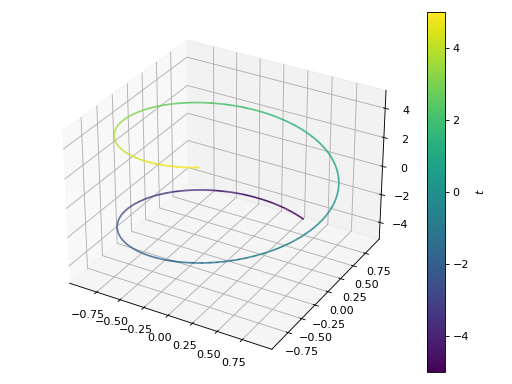
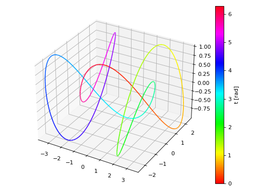
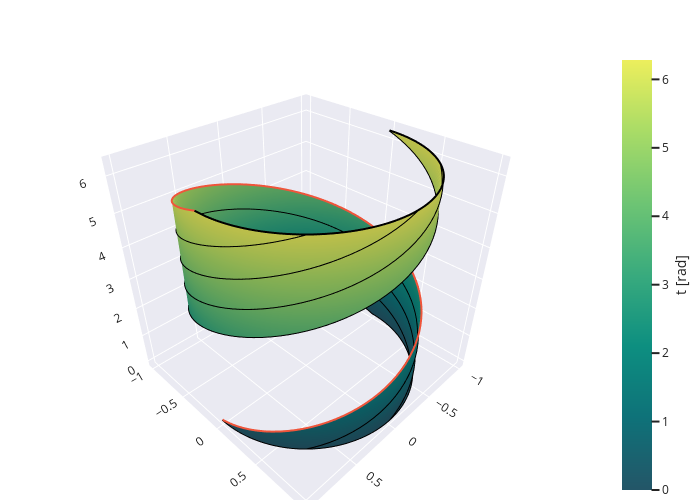
Customize the appearance by setting a label to the colorbar, changing the colormap, the line width, and the ticks on the colorbar.
>>> graphics(
...     line_parametric_3d(
...         3 * sin(t) + 2 * sin(3 * t), cos(t) - 2 * cos(3 * t), cos(5 * t),
...         (t, 0, 2 * pi), "t [rad]", {"cmap": "hsv", "lw": 1.5},
...         colorbar_ticks_formatter=multiples_of_pi_over_2()
...     )
... )
Plot object containing:
[0]: 3D parametric cartesian line: (3*sin(t) + 2*sin(3*t), cos(t) - 2*cos(3*t), cos(5*t)) for t over (0, 2*pi)
(
Source code,png)
Plot multiple parametric 3D lines with different ranges:
>>> a, b, n = 2, 1, 4
>>> p, r, s = symbols("p r s")
>>> xp = a * cos(p) * cos(n * p)
>>> yp = a * sin(p) * cos(n * p)
>>> zp = b * cos(n * p)**2 + pi
>>> xr = root(r, 3) * cos(r)
>>> yr = root(r, 3) * sin(r)
>>> zr = 0
>>> graphics(
...     line_parametric_3d(
...         xp, yp, zp, (p, 0, pi if n % 2 == 1 else 2 * pi), "petals",
...         use_cm=False),
...     line_parametric_3d(xr, yr, zr, (r, 0, 6*pi), "roots",
...         use_cm=False),
...     line_parametric_3d(-sin(s)/3, 0, s, (s, 0, pi), "stem",
...         use_cm=False)
... )
Plot object containing:
[0]: 3D parametric cartesian line: (2*cos(p)*cos(4*p), 2*sin(p)*cos(4*p), cos(4*p)**2 + pi) for p over (0, 2*pi)
[1]: 3D parametric cartesian line: (r**(1/3)*cos(r), r**(1/3)*sin(r), 0) for r over (0, 6*pi)
[2]: 3D parametric cartesian line: (-sin(s)/3, 0, s) for s over (0, pi)
(
Source code,png)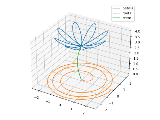
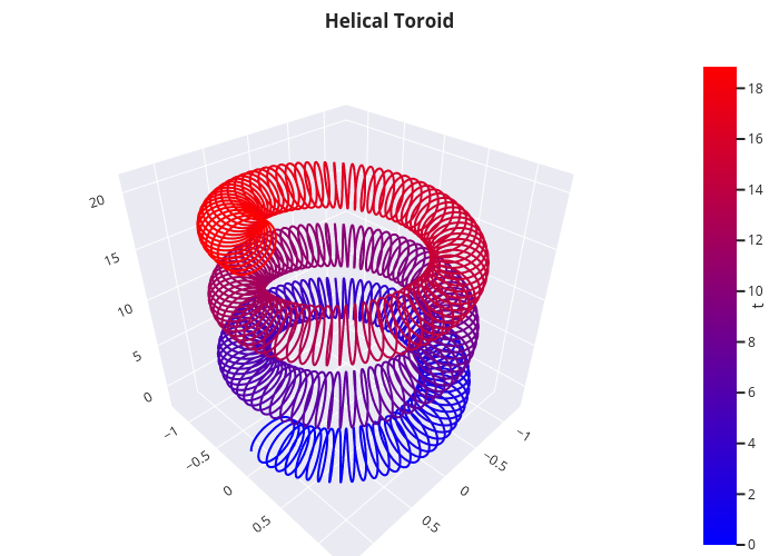
Plotting a numerical function instead of a symbolic expression, using Plotly:
from spb import *
import numpy as np
fx = lambda t: (1 + 0.25 * np.cos(75 * t)) * np.cos(t)
fy = lambda t: (1 + 0.25 * np.cos(75 * t)) * np.sin(t)
fz = lambda t: t + 2 * np.sin(75 * t)
graphics(
    line_parametric_3d(fx, fy, fz, ("t", 0, 6 * np.pi),
        rendering_kw={"line": {"colorscale": "bluered"}}, n=1e04),
    title="Helical Toroid", backend=PB)
(Source code, png)
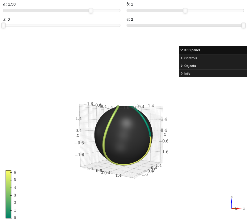
Interactive-widget plot of the parametric line over a tennis ball. Refer to the interactive sub-module documentation to learn more about the
paramsdictionary. This plot illustrates:combining together different plots.
the use of
prange(parametric plotting range).the use of the
paramsdictionary to specify sliders in their basic form: (default, min, max).
from sympy import *
from spb import *
import k3d
a, b, s, e, t = symbols("a, b, s, e, t")
c = 2 * sqrt(a * b)
r = a + b
params = {
    a: (1.5, 0, 2),
    b: (1, 0, 2),
    s: (0, 0, 2),
    e: (2, 0, 2)
}
graphics(
    surface_revolution(
        (r * cos(t), r * sin(t)), (t, 0, pi),
        params=params, n=50, parallel_axis="x", show_curve=False,
        rendering_kw={"color":0x353535},
        force_real_eval=True
    ),
    line_parametric_3d(
        a * cos(t) + b * cos(3 * t),
        a * sin(t) - b * sin(3 * t),
        c * sin(2 * t), prange(t, s*pi, e*pi),
        rendering_kw={"color_map": k3d.matplotlib_color_maps.Summer},
        params=params
    ),
    backend=KB
)

- spb.graphics.functions_3d.list_3d(list_x, list_y, list_z, label=None, rendering_kw=None, **kwargs)[source]
Plots lists of coordinates in 3D space.
- Parameters:
- list_x
Coordinates for the x-axis. It can be a list or a numper array.
- list_y
Coordinates for the y-axis. It can be a list or a numper array.
- list_z
Coordinates for the z-axis. It can be a list or a numper array.
- labelstr
Set the label associated to this series, which will be eventually shown on the legend or colorbar.
- rendering_kwdict
A dictionary of keyword arguments to be passed to the renderers in order to further customize the appearance of the line. Here are some useful links for the supported plotting libraries:
Matplotlib:
for solid lines: https://matplotlib.org/stable/api/_as_gen/matplotlib.pyplot.plot.html
for colormap-based lines: https://matplotlib.org/stable/api/collections_api.html#matplotlib.collections.LineCollection
for scatters: https://matplotlib.org/stable/api/_as_gen/matplotlib.pyplot.scatter.html
Bokeh:
- color_funccallable
A color function to be applied to the numerical data. It can be:
None: no color function.
callable: a function accepting:
no arguments: this can be used to return an array of precomputed values.
three arguments, the x, y, z coordinates.
- colorbarbool
Toggle the visibility of the colorbar associated to the current data series. Note that a colorbar is only visible if
use_cm=Trueandcolor_funcis not None. Default value: True.- colorbar_ticks_formattertick_formatter_multiples_of
An object of type
tick_formatter_multiples_ofwhich will be used to place tick values on the colorbar at each multiple of a specified quantity. This only works when use_cm=True.- is_filledbool
Whether scatter’s markers are filled or void. Default value: True.
- is_scatterbool
If True it represent a scatter plot, otherwise a continuous line. Default value: False.
- line_color
For back-compatibility with old sympy.plotting. Use
rendering_kwin order to fully customize the appearance of the line/scatter.- paramsdict, optional
A dictionary mapping symbols to parameters. If provided, this dictionary enables the interactive-widgets plot.
When calling a plotting function, the parameter can be specified with:
a widget from the
ipywidgetsmodule.a widget from the
panelmodule.- a tuple of the form:
(default, min, max, N, tick_format, label, spacing), which will instantiate a
ipywidgets.widgets.widget_float.FloatSlideror aipywidgets.widgets.widget_float.FloatLogSlider, depending on the spacing strategy. In particular:- default, min, maxfloat
Default value, minimum value and maximum value of the slider, respectively. Must be finite numbers. The order of these 3 numbers is not important: the module will figure it out which is what.
- Nint, optional
Number of steps of the slider.
- tick_formatstr or None, optional
Provide a formatter for the tick value of the slider. Default to
".2f".
- label: str, optional
Custom text associated to the slider.
- spacingstr, optional
Specify the discretization spacing. Default to
"linear", can be changed to"log".
Notes:
parameters cannot be linked together (ie, one parameter cannot depend on another one).
If a widget returns multiple numerical values (like
panel.widgets.slider.RangeSlideroripywidgets.widgets.widget_float.FloatRangeSlider), then a corresponding number of symbols must be provided.
Here follows a couple of examples. If
imodule="panel":import panel as pn params = { a: (1, 0, 5), # slider from 0 to 5, with default value of 1 b: pn.widgets.FloatSlider(value=1, start=0, end=5), # same slider as above (c, d): pn.widgets.RangeSlider(value=(-1, 1), start=-3, end=3, step=0.1) }
Or with
imodule="ipywidgets":import ipywidgets as w params = { a: (1, 0, 5), # slider from 0 to 5, with default value of 1 b: w.FloatSlider(value=1, min=0, max=5), # same slider as above (c, d): w.FloatRangeSlider(value=(-1, 1), min=-3, max=3, step=0.1) }
When instantiating a data series directly,
paramsmust be a dictionary mapping symbols to numerical values.Let
seriesbe any data series. Thenseries.paramsreturns a dictionary mapping symbols to numerical values.- show_in_legendbool
Toggle the visibility of the data series on the legend. Default value: True.
- stepsNoneType, bool, str
If set, it connects consecutive points with steps rather than straight segments. Possible options: [‘pre’, ‘post’, ‘mid’, True, False, None] Default value: False.
- txcallable
Numerical transformation function to be applied to the data on the x-axis.
- tycallable
Numerical transformation function to be applied to the data on the y-axis.
- tzcallable
Numerical transformation function to be applied to the data on the z-axis.
- unwrapbool, dict
Whether to use numpy.unwrap() on the computed coordinates in order to get rid of discontinuities. It can be:
False: do not use
np.unwrap().True: use
np.unwrap()with default keyword arguments.dictionary of keyword arguments passed to
np.unwrap().
- use_cmbool
Toggle the use of a colormap. By default, some series might use a colormap to display the necessary data. Setting this attribute to False will inform the associated renderer to use solid color. Related parameters:
color_func. Default value: False.
- Returns:
- serieslist
A list containing one instance of
List3DSeries.
Examples
>>> from sympy import *
>>> from spb import *
>>> import numpy as np
Plot the coordinates of a single function:
>>> z = np.linspace(0, 6*np.pi, 100)
>>> x = z * np.cos(z)
>>> y = z * np.sin(z)
>>> graphics(list_3d(x, y, z))
Plot object containing:
[0]: 3D list plot
(
Source code,png)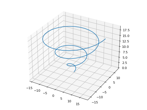
Plotting multiple functions with custom rendering keywords:
>>> graphics(
...     list_3d(x, y, z, "A"),
...     list_3d(x, y, -z, "B", {"linestyle": "--"}))
Plot object containing:
[0]: 3D list plot
[1]: 3D list plot
(
Source code,png)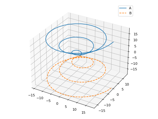
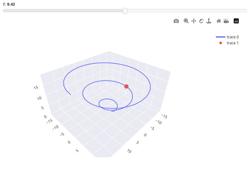
Interactive-widget plot of a dot following a path. Refer to the interactive sub-module documentation to learn more about the
paramsdictionary.from sympy import * from spb import * import numpy as np t = symbols("t") z = np.linspace(0, 6*np.pi, 100) x = z * np.cos(z) y = z * np.sin(z) graphics( list_3d(x, y, z, is_scatter=False), list_3d(t * cos(t), t * sin(t), t, params={t: (3*pi, 0, 6*pi)}, is_scatter=True), backend=PB )
- spb.graphics.functions_3d.surface(expr, range_x=None, range_y=None, label=None, rendering_kw=None, colorbar=True, use_cm=False, **kwargs)[source]
Creates the surface of a function of 2 variables.
- Parameters:
- expr
The expression representing the function of two variables to be plotted. It can be a:
Symbolic expression.
Numerical function of two variable, supporting vectorization. In this case the following keyword arguments are not supported:
params.
- range_xtuple, Tuple
A 3-tuple (symb, min, max) denoting the range of the x variable. Default values: min=-10 and max=10.
- range_ytuple, Tuple
A 3-tuple (symb, min, max) denoting the range of the y variable. Default values: min=-10 and max=10.
- labelstr
Set the label associated to this series, which will be eventually shown on the legend or colorbar.
- rendering_kwdict
A dictionary of keyword arguments to be passed to the renderers in order to further customize the appearance of the surface. Here are some useful links for the supported plotting libraries:
K3D-Jupyter: look at the documentation of k3d.mesh.
- colorbarbool
Toggle the visibility of the colorbar associated to the current data series. Note that a colorbar is only visible if
use_cm=Trueandcolor_funcis not None. Default value: True.- use_cmbool
Toggle the use of a colormap. By default, some series might use a colormap to display the necessary data. Setting this attribute to False will inform the associated renderer to use solid color. Related parameters:
color_func. Default value: False.- color_func
Define a custom color mapping. It can either be:
A numerical function supporting vectorization. The arity can be:
2 arguments:
f(x, y)wherex, yare the coordinates of the points.3 arguments:
f(x, y, z)wherex, y, zare the coordinates of the points.
A symbolic expression having at most as many free symbols as
expr.None: the default value (color mapping according to the z coordinate).
- colorbar_ticks_formattertick_formatter_multiples_of
An object of type
tick_formatter_multiples_ofwhich will be used to place tick values on the colorbar at each multiple of a specified quantity. This only works when use_cm=True.- force_real_evalbool
By default, numerical evaluation is performed over complex numbers, which is slower but produces correct results. However, when the symbolic expression is converted to a numerical function with lambdify, the resulting function may not like to be evaluated over complex numbers. In such cases, forcing the evaluation to be performed over real numbers might be a good choice. The plotting module should be able to detect such occurences and automatically activate this option. If that is not the case, or evaluation performance is of paramount importance, set this parameter to True, but be aware that it might produce wrong results. Default value: False.
- is_polarbool
If True, requests a polar discretization. In this case,
range_xrepresents the radius, whilerange_yrepresents the angle. Default value: False.- modules
Specify the evaluation modules to be used by lambdify. If not specified, the evaluation will be done with NumPy/SciPy.
- n1int
Number of discretization points along the x-axis to be used in the evaluation. Related parameters:
xscale. It must be: 2 ≤ n1 < ∞. Default value: 100.- n2int
Number of discretization points along the y-axis to be used in the evaluation. Related parameters:
yscale. It must be: 2 ≤ n2 < ∞. Default value: 100.- only_integersbool
Discretize the domain using only integer numbers. When this parameter is True, the number of discretization points is choosen by the algorithm. Default value: False.
- paramsdict, optional
A dictionary mapping symbols to parameters. If provided, this dictionary enables the interactive-widgets plot.
When calling a plotting function, the parameter can be specified with:
a widget from the
ipywidgetsmodule.a widget from the
panelmodule.- a tuple of the form:
(default, min, max, N, tick_format, label, spacing), which will instantiate a
ipywidgets.widgets.widget_float.FloatSlideror aipywidgets.widgets.widget_float.FloatLogSlider, depending on the spacing strategy. In particular:- default, min, maxfloat
Default value, minimum value and maximum value of the slider, respectively. Must be finite numbers. The order of these 3 numbers is not important: the module will figure it out which is what.
- Nint, optional
Number of steps of the slider.
- tick_formatstr or None, optional
Provide a formatter for the tick value of the slider. Default to
".2f".
- label: str, optional
Custom text associated to the slider.
- spacingstr, optional
Specify the discretization spacing. Default to
"linear", can be changed to"log".
Notes:
parameters cannot be linked together (ie, one parameter cannot depend on another one).
If a widget returns multiple numerical values (like
panel.widgets.slider.RangeSlideroripywidgets.widgets.widget_float.FloatRangeSlider), then a corresponding number of symbols must be provided.
Here follows a couple of examples. If
imodule="panel":import panel as pn params = { a: (1, 0, 5), # slider from 0 to 5, with default value of 1 b: pn.widgets.FloatSlider(value=1, start=0, end=5), # same slider as above (c, d): pn.widgets.RangeSlider(value=(-1, 1), start=-3, end=3, step=0.1) }
Or with
imodule="ipywidgets":import ipywidgets as w params = { a: (1, 0, 5), # slider from 0 to 5, with default value of 1 b: w.FloatSlider(value=1, min=0, max=5), # same slider as above (c, d): w.FloatRangeSlider(value=(-1, 1), min=-3, max=3, step=0.1) }
When instantiating a data series directly,
paramsmust be a dictionary mapping symbols to numerical values.Let
seriesbe any data series. Thenseries.paramsreturns a dictionary mapping symbols to numerical values.- show_in_legendbool
Toggle the visibility of the data series on the legend. Default value: True.
- sum_boundint
When plotting sums, the expression will be pre-processed in order to replace lower/upper bounds set to +/- infinity with this +/- numerical value. Note: the higher this number, the slower the evaluation, but the more accurate the plot. It must be: 0 ≤ sum_bound < ∞. Default value: 1000.
- surface_color
For back-compatibility with old sympy.plotting. Use
rendering_kwin order to fully customize the appearance of the surface.- txcallable
Numerical transformation function to be applied to the data on the x-axis.
- tycallable
Numerical transformation function to be applied to the data on the y-axis.
- tzcallable
Numerical transformation function to be applied to the data on the z-axis.
- wf_n1, wf_n2int, optional
Number of wireframe lines along the two ranges, respectively. Default to 10. Note that increasing this number might considerably slow down the plot’s creation. Related parameter:
wireframe.- wf_npointsint or None, optional
Number of discretization points for the wireframe lines. Default to None, meaning that each wireframe line will have
n1orn2number of points, depending on the line direction. Related parameter:wireframe.- wf_rendering_kwdict, optional
A dictionary of keywords/values which is passed to the backend’s function to customize the appearance of wireframe lines. Related parameter:
wireframe.- wireframeboolean, optional
Enable or disable a wireframe over the surface. Depending on the number of wireframe lines (see
wf_n1andwf_n2), activating this option might add a considerable overhead during the plot’s creation. Default to False (disabled).- xscalestr
Discretization strategy along the x-direction. Related parameters:
n1. Possible options: [‘linear’, ‘log’] Default value: ‘linear’.- yscalestr
Discretization strategy along the y-direction. Related parameters:
n2. Possible options: [‘linear’, ‘log’] Default value: ‘linear’.
- Returns:
- serieslist
A list containing one instance of
SurfaceOver2DRangeSeriesand possibly multiple instances ofParametric3DLineSeries, ifwireframe=True.
See also
Examples
>>> from sympy import symbols, cos, sin, pi, exp
>>> from spb import *
>>> x, y = symbols('x y')
Single plot with Matplotlib, with ticks formatted as multiples of pi/2.
>>> graphics(
...     surface(cos((x**2 + y**2)), (x, -pi, pi), (y, -pi, pi)),
...     x_ticks_formatter=multiples_of_pi_over_2(),
...     y_ticks_formatter=multiples_of_pi_over_2(),
... )
Plot object containing:
[0]: cartesian surface: cos(x**2 + y**2) for x over (-pi, pi) and y over (-pi, pi)
(
Source code,png)
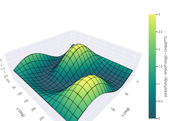
Single plot with Plotly, illustrating how to apply:
a color map: by default, it will map colors to the z values.
wireframe lines to better understand the discretization and curvature.
transformation to the discretized ranges in order to convert radians to degrees.
custom aspect ratio with Plotly.
from sympy import symbols, sin, cos, pi
from spb import *
import numpy as np
x, y = symbols("x, y")
expr = (cos(x) + sin(x) * sin(y) - sin(x) * cos(y))**2
graphics(
    surface(expr, (x, 0, pi), (y, 0, 2 * pi), use_cm=True,
        tx=np.rad2deg, ty=np.rad2deg,
        wireframe=True, wf_n1=20, wf_n2=20),
    backend=PB, xlabel="x [deg]", ylabel="y [deg]",
    aspect=dict(x=1.5, y=1.5, z=0.5))
(Source code, png)
Multiple plots with same range using color maps. By default, colors are mapped to the z values:
>>> graphics(
...     surface(x*y, (x, -5, 5), (y, -5, 5), use_cm=True),
...     surface(-x*y, (x, -5, 5), (y, -5, 5), use_cm=True))
Plot object containing:
[0]: cartesian surface: x*y for x over (-5, 5) and y over (-5, 5)
[1]: cartesian surface: -x*y for x over (-5, 5) and y over (-5, 5)
(
Source code,png)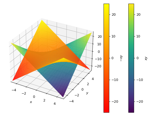
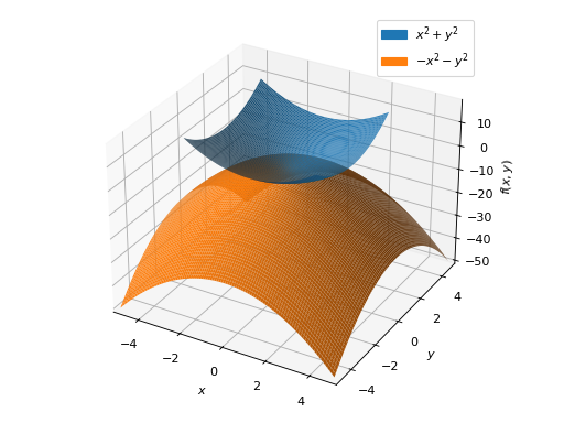
Multiple plots with different ranges and solid colors.
>>> f = x**2 + y**2
>>> graphics(
...     surface(f, (x, -3, 3), (y, -3, 3)),
...     surface(-f, (x, -5, 5), (y, -5, 5)))
Plot object containing:
[0]: cartesian surface: x**2 + y**2 for x over (-3, 3) and y over (-3, 3)
[1]: cartesian surface: -x**2 - y**2 for x over (-5, 5) and y over (-5, 5)
(
Source code,png)
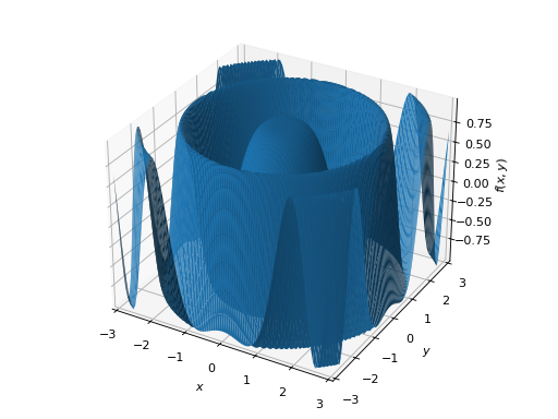
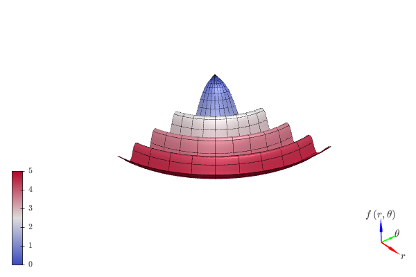
Single plot with a polar discretization, a color function mapping a colormap to the radius. Note that the same result can be achieved with
plot3d_revolution.from sympy import * from spb import * import numpy as np r, theta = symbols("r, theta") expr = cos(r**2) * exp(-r / 3) graphics( surface(expr, (r, 0, 5), (theta, 1.6 * pi, 2 * pi), use_cm=True, color_func=lambda x, y, z: np.sqrt(x**2 + y**2), is_polar=True, wireframe=True, wf_n1=30, wf_n2=10, wf_rendering_kw={"width": 0.005}), backend=KB, legend=True, grid=False)

Plotting a numerical function instead of a symbolic expression:
>>> graphics(
...     surface(lambda x, y: x * np.exp(-x**2 - y**2),
...         ("x", -3, 3), ("y", -3, 3), use_cm=True))
(
Source code,png)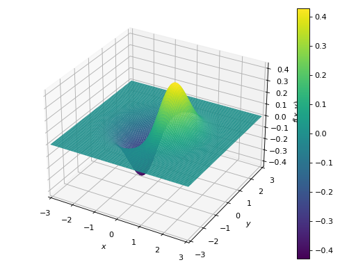
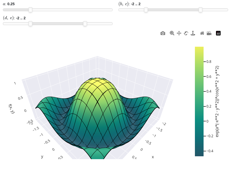
Interactive-widget plot. Refer to the interactive sub-module documentation to learn more about the
paramsdictionary. This plot illustrates:the use of
prange(parametric plotting range).the use of the
paramsdictionary to specify sliders in their basic form: (default, min, max).the use of
panel.widgets.slider.RangeSlider, which is a 2-values widget.
from sympy import *
from spb import *
import panel as pn
x, y, a, b, c, d, e = symbols("x y a b c d e")
graphics(
    surface(
        cos(x**2 + y**2) * exp(-(x**2 + y**2) * a),
        prange(x, b, c), prange(y, d, e),
        params={
            a: (0.25, 0, 1),
            (b, c): pn.widgets.RangeSlider(
                value=(-2, 2), start=-4, end=4, step=0.1),
            (d, e): pn.widgets.RangeSlider(
                value=(-2, 2), start=-4, end=4, step=0.1),
        },
        use_cm=True, n=100,
        wireframe=True, wf_n1=15, wf_n2=15),
    backend=PB, aspect=dict(x=1.5, y=1.5, z=0.75))

- spb.graphics.functions_3d.surface_parametric(expr_x, expr_y, expr_z, range_u=None, range_v=None, label=None, rendering_kw=None, **kwargs)[source]
Creates a 3D parametric surface.
- Parameters:
- expr_x
The expression representing the component along the x-axis of the parametric function. It can be a:
Symbolic expression.
Numerical function of two variable, f(u, v), supporting vectorization. In this case the following keyword arguments are not supported:
params.
- expr_y
The expression representing the component along the y-axis of the parametric function. It can be a:
Symbolic expression.
Numerical function of two variable, f(u, v), supporting vectorization. In this case the following keyword arguments are not supported:
params.
- expr_z
The expression representing the component along the z-axis of the parametric function. It can be a:
Symbolic expression.
Numerical function of two variable, f(u, v), supporting vectorization. In this case the following keyword arguments are not supported:
params.
- range_utuple, Tuple
A 3-tuple (symb, min, max) denoting the range of the u parameter. Default values: min=-10 and max=10.
- range_vtuple, Tuple
A 3-tuple (symb, min, max) denoting the range of the v parameter. Default values: min=-10 and max=10.
- labelstr
Set the label associated to this series, which will be eventually shown on the legend or colorbar.
- rendering_kwdict
A dictionary of keyword arguments to be passed to the renderers in order to further customize the appearance of the surface. Here are some useful links for the supported plotting libraries:
K3D-Jupyter: look at the documentation of k3d.mesh.
- color_func
Define the surface color mapping when use_cm=True. It can either be:
None: the default value (color mapping according to the z coordinate).
A numerical function supporting vectorization. The arity can be:
1 argument:
f(u), whereuis the first parameter.2 arguments:
f(u, v)whereu, vare the parameters.3 arguments:
f(x, y, z)wherex, y, zare the coordinates of the points.5 arguments:
f(x, y, z, u, v).
A symbolic expression having at most as many free symbols as
expr_xorexpr_yorexpr_z.
- colorbarbool
Toggle the visibility of the colorbar associated to the current data series. Note that a colorbar is only visible if
use_cm=Trueandcolor_funcis not None. Default value: True.- colorbar_ticks_formattertick_formatter_multiples_of
An object of type
tick_formatter_multiples_ofwhich will be used to place tick values on the colorbar at each multiple of a specified quantity. This only works when use_cm=True.- force_real_evalbool
By default, numerical evaluation is performed over complex numbers, which is slower but produces correct results. However, when the symbolic expression is converted to a numerical function with lambdify, the resulting function may not like to be evaluated over complex numbers. In such cases, forcing the evaluation to be performed over real numbers might be a good choice. The plotting module should be able to detect such occurences and automatically activate this option. If that is not the case, or evaluation performance is of paramount importance, set this parameter to True, but be aware that it might produce wrong results. Default value: False.
- modules
Specify the evaluation modules to be used by lambdify. If not specified, the evaluation will be done with NumPy/SciPy.
- n1int
Number of discretization points along the first parameter to be used in the evaluation. Related parameters:
xscale. It must be: 2 ≤ n1 < ∞. Default value: 100.- n2int
Number of discretization points along the second parameter to be used in the evaluation. Related parameters:
yscale. It must be: 2 ≤ n2 < ∞. Default value: 100.- only_integersbool
Discretize the domain using only integer numbers. When this parameter is True, the number of discretization points is choosen by the algorithm. Default value: False.
- paramsdict, optional
A dictionary mapping symbols to parameters. If provided, this dictionary enables the interactive-widgets plot.
When calling a plotting function, the parameter can be specified with:
a widget from the
ipywidgetsmodule.a widget from the
panelmodule.- a tuple of the form:
(default, min, max, N, tick_format, label, spacing), which will instantiate a
ipywidgets.widgets.widget_float.FloatSlideror aipywidgets.widgets.widget_float.FloatLogSlider, depending on the spacing strategy. In particular:- default, min, maxfloat
Default value, minimum value and maximum value of the slider, respectively. Must be finite numbers. The order of these 3 numbers is not important: the module will figure it out which is what.
- Nint, optional
Number of steps of the slider.
- tick_formatstr or None, optional
Provide a formatter for the tick value of the slider. Default to
".2f".
- label: str, optional
Custom text associated to the slider.
- spacingstr, optional
Specify the discretization spacing. Default to
"linear", can be changed to"log".
Notes:
parameters cannot be linked together (ie, one parameter cannot depend on another one).
If a widget returns multiple numerical values (like
panel.widgets.slider.RangeSlideroripywidgets.widgets.widget_float.FloatRangeSlider), then a corresponding number of symbols must be provided.
Here follows a couple of examples. If
imodule="panel":import panel as pn params = { a: (1, 0, 5), # slider from 0 to 5, with default value of 1 b: pn.widgets.FloatSlider(value=1, start=0, end=5), # same slider as above (c, d): pn.widgets.RangeSlider(value=(-1, 1), start=-3, end=3, step=0.1) }
Or with
imodule="ipywidgets":import ipywidgets as w params = { a: (1, 0, 5), # slider from 0 to 5, with default value of 1 b: w.FloatSlider(value=1, min=0, max=5), # same slider as above (c, d): w.FloatRangeSlider(value=(-1, 1), min=-3, max=3, step=0.1) }
When instantiating a data series directly,
paramsmust be a dictionary mapping symbols to numerical values.Let
seriesbe any data series. Thenseries.paramsreturns a dictionary mapping symbols to numerical values.- show_in_legendbool
Toggle the visibility of the data series on the legend. Default value: True.
- sum_boundint
When plotting sums, the expression will be pre-processed in order to replace lower/upper bounds set to +/- infinity with this +/- numerical value. Note: the higher this number, the slower the evaluation, but the more accurate the plot. It must be: 0 ≤ sum_bound < ∞. Default value: 1000.
- surface_color
For back-compatibility with old sympy.plotting. Use
rendering_kwin order to fully customize the appearance of the surface.- txcallable
Numerical transformation function to be applied to the data on the x-axis.
- tycallable
Numerical transformation function to be applied to the data on the y-axis.
- tzcallable
Numerical transformation function to be applied to the data on the z-axis.
- use_cmbool
Toggle the use of a colormap. By default, some series might use a colormap to display the necessary data. Setting this attribute to False will inform the associated renderer to use solid color. Related parameters:
color_func. Default value: False.- wf_n1, wf_n2int, optional
Number of wireframe lines along the two ranges, respectively. Default to 10. Note that increasing this number might considerably slow down the plot’s creation. Related parameter:
wireframe.- wf_npointsint or None, optional
Number of discretization points for the wireframe lines. Default to None, meaning that each wireframe line will have
n1orn2number of points, depending on the line direction. Related parameter:wireframe.- wf_rendering_kwdict, optional
A dictionary of keywords/values which is passed to the backend’s function to customize the appearance of wireframe lines. Related parameter:
wireframe.- wireframeboolean, optional
Enable or disable a wireframe over the surface. Depending on the number of wireframe lines (see
wf_n1andwf_n2), activating this option might add a considerable overhead during the plot’s creation. Default to False (disabled).- xscalestr
Discretization strategy along the first parameter. Related parameters:
n1. Possible options: [‘linear’, ‘log’] Default value: ‘linear’.- yscalestr
Discretization strategy along the second parameter. Related parameters:
n2. Possible options: [‘linear’, ‘log’] Default value: ‘linear’.
- Returns:
- serieslist
A list containing one instance of
ParametricSurfaceSeriesand possibly multiple instances ofParametric3DLineSeries, ifwireframe=True.
See also
Examples
>>> from sympy import symbols, cos, sin, pi, I, sqrt, atan2, re, im
>>> from spb import *
>>> u, v = symbols('u v')
Plot a parametric surface:
>>> graphics(
...     surface_parametric(
...         u * cos(v), u * sin(v), u * cos(4 * v) / 2,
...         (u, 0, pi), (v, 0, 2*pi), use_cm=False),
...     title="Sinusoidal Cone")
Plot object containing:
[0]: parametric cartesian surface: (u*cos(v), u*sin(v), u*cos(4*v)/2) for u over (0, pi) and v over (0, 2*pi)
(
Source code,png)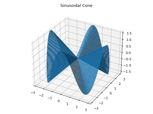
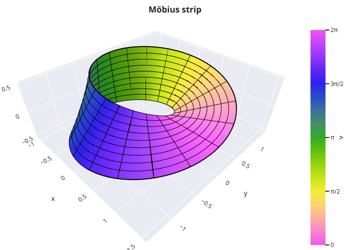
Customize the appearance of the surface by changing the colormap. Apply a color function mapping the v values. Activate the wireframe to better visualize the parameterization.
from sympy import *
from spb import *
var("u, v")

x = (1 + v / 2 * cos(u / 2)) * cos(u)
y = (1 + v / 2 * cos(u / 2)) * sin(u)
z = v / 2 * sin(u / 2)
graphics(
surface_parametric(x, y, z, (u, 0, 2*pi), (v, -1, 1),
    "v", {"colorscale": "mygbm"},
    use_cm=True, color_func=lambda u, v: u,
    wireframe=True, wf_n1=20,
    colorbar_ticks_formatter=multiples_of_pi_over_2(label="π")
),
xlabel="x", ylabel="y", zlabel="z",
backend=PB, title="Möbius strip")
(Source code, png)
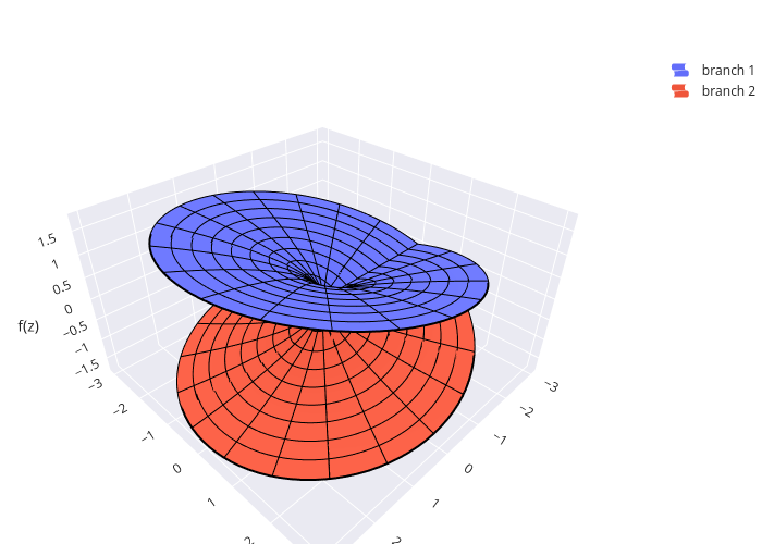
Riemann surfaces of the real part of the multivalued function z**n, using Plotly:
from sympy import symbols, sqrt, re, im, pi, atan2, sin, cos, I
from spb import *
r, theta, x, y = symbols("r, theta, x, y", real=True)
mag = lambda z: sqrt(re(z)**2 + im(z)**2)
phase = lambda z, k=0: atan2(im(z), re(z)) + 2 * k * pi
n = 2 # exponent (integer)
z = x + I * y # cartesian
d = {x: r * cos(theta), y: r * sin(theta)} # cartesian to polar
branches = [(mag(z)**(1 / n) * cos(phase(z, i) / n)).subs(d)
    for i in range(n)]
exprs = [(r * cos(theta), r * sin(theta), rb) for rb in branches]
series = [
    surface_parametric(*e, (r, 0, 3), (theta, -pi, pi),
        label="branch %s" % (i + 1), wireframe=True, wf_n2=20)
    for i, e in enumerate(exprs)]
graphics(*series, backend=PB, zlabel="f(z)")
(Source code, png)
Plotting a numerical function instead of a symbolic expression.
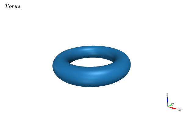
from spb import *
import numpy as np
fx = lambda u, v: (4 + np.cos(u)) * np.cos(v)
fy = lambda u, v: (4 + np.cos(u)) * np.sin(v)
fz = lambda u, v: np.sin(u)
graphics(
    surface_parametric(fx, fy, fz, ("u", 0, 2 * np.pi),
        ("v", 0, 2 * np.pi)),
    zlim=(-2.5, 2.5), title="Torus", backend=KB, grid=False)
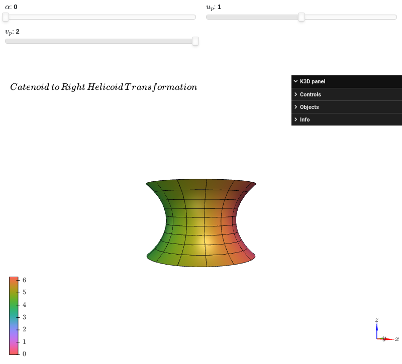
Interactive-widget plot. Refer to the interactive sub-module documentation to learn more about the
paramsdictionary. This plot illustrates:the use of
prange(parametric plotting range).the use of the
paramsdictionary to specify sliders in their basic form: (default, min, max).
from sympy import *
from spb import *
import k3d
alpha, u, v, up, vp = symbols("alpha u v u_p v_p")
graphics(
    surface_parametric(
        exp(u) * cos(v - alpha) / 2 + exp(-u) * cos(v + alpha) / 2,
        exp(u) * sin(v - alpha) / 2 + exp(-u) * sin(v + alpha) / 2,
        cos(alpha) * u + sin(alpha) * v,
        prange(u, -up, up), prange(v, 0, vp * pi),
        n=50, use_cm=True, color_func=lambda u, v: v,
        rendering_kw={"color_map": k3d.colormaps.paraview_color_maps.Hue_L60},
        wireframe=True, wf_n2=15, wf_rendering_kw={"width": 0.005},
        params={
            alpha: (0, 0, pi),
            up: (1, 0, 2),
            vp: (2, 0, 2),
        }),
    backend=KB, grid=False,
    title="Catenoid \, to \, Right \, Helicoid \, Transformation"
)
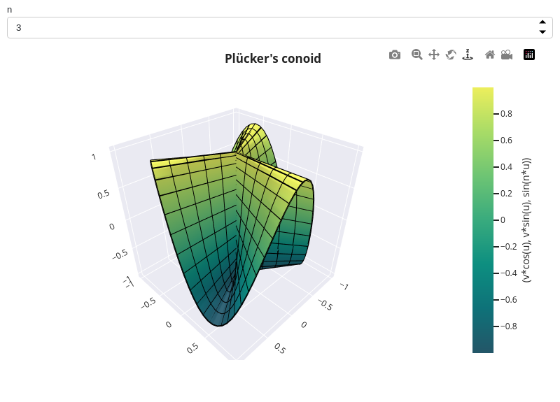
Interactive-widget plot. Refer to the interactive sub-module documentation to learn more about the
paramsdictionary. Note that the plot’s creation might be slow due to the wireframe lines.from sympy import * from spb import * import panel as pn n, u, v = symbols("n, u, v") x = v * cos(u) y = v * sin(u) z = sin(n * u) graphics( surface_parametric(x, y, z, (u, 0, 2*pi), (v, -1, 0), params = { n: pn.widgets.IntInput(value=3, name="n") }, use_cm=True, wireframe=True, wf_n1=75, wf_n2=6), backend=PB, title="Plücker's conoid", imodule="panel" )

- spb.graphics.functions_3d.surface_revolution(curve, range_t, range_phi=None, axis=(0, 0), parallel_axis='z', show_curve=False, curve_kw={}, **kwargs)[source]
Creates a surface of revolution by rotating a curve around an axis of rotation.
- Parameters:
- curveExpr, list ortuple of 2 or 3 elements
The curve to be revolved, which can be either:
a symbolic expression
a 2-tuple representing a parametric curve in 2D space
a 3-tuple representing a parametric curve in 3D space
- range_ttuple
A 3-tuple (symbol, min, max) denoting the range of the parameter of the curve.
- range_phituple
A 3-tuple (symbol, min, max) denoting the range of the azimuthal angle where the curve will be revolved. Default to
(phi, 0, 2*pi).- axistuple
A 2-tuple (coord1, coord2) that specifies the position of the rotation axis. Depending on the value of
parallel_axis:"x": the rotation axis intersects the YZ plane at (coord1, coord2)."y": the rotation axis intersects the XZ plane at (coord1, coord2)."z": the rotation axis intersects the XY plane at (coord1, coord2).
Default to
(0, 0).- parallel_axisstr
Specify the axis parallel to the axis of rotation. Must be one of the following options: “x”, “y” or “z”. Default to “z”.
- show_curvebool
Add the initial curve to the plot. Default to False.
- curve_kwdict
A dictionary of options that will be passed to
plot3d_parametric_lineifshow_curve=Truein order to customize the appearance of the initial curve. Refer to its documentation for more information.- color_func
Define the surface color mapping when use_cm=True. It can either be:
None: the default value (color mapping according to the z coordinate).
A numerical function supporting vectorization. The arity can be:
1 argument:
f(u), whereuis the first parameter.2 arguments:
f(u, v)whereu, vare the parameters.3 arguments:
f(x, y, z)wherex, y, zare the coordinates of the points.5 arguments:
f(x, y, z, u, v).
A symbolic expression having at most as many free symbols as
expr_xorexpr_yorexpr_z.
- colorbarbool
Toggle the visibility of the colorbar associated to the current data series. Note that a colorbar is only visible if
use_cm=Trueandcolor_funcis not None. Default value: True.- colorbar_ticks_formattertick_formatter_multiples_of
An object of type
tick_formatter_multiples_ofwhich will be used to place tick values on the colorbar at each multiple of a specified quantity. This only works when use_cm=True.- force_real_evalbool
By default, numerical evaluation is performed over complex numbers, which is slower but produces correct results. However, when the symbolic expression is converted to a numerical function with lambdify, the resulting function may not like to be evaluated over complex numbers. In such cases, forcing the evaluation to be performed over real numbers might be a good choice. The plotting module should be able to detect such occurences and automatically activate this option. If that is not the case, or evaluation performance is of paramount importance, set this parameter to True, but be aware that it might produce wrong results. Default value: False.
- labelstr
Set the label associated to this series, which will be eventually shown on the legend or colorbar.
- modules
Specify the evaluation modules to be used by lambdify. If not specified, the evaluation will be done with NumPy/SciPy.
- n1int
Number of discretization points along the first parameter to be used in the evaluation. Related parameters:
xscale. It must be: 2 ≤ n1 < ∞. Default value: 100.- n2int
Number of discretization points along the second parameter to be used in the evaluation. Related parameters:
yscale. It must be: 2 ≤ n2 < ∞. Default value: 100.- only_integersbool
Discretize the domain using only integer numbers. When this parameter is True, the number of discretization points is choosen by the algorithm. Default value: False.
- paramsdict, optional
A dictionary mapping symbols to parameters. If provided, this dictionary enables the interactive-widgets plot.
When calling a plotting function, the parameter can be specified with:
a widget from the
ipywidgetsmodule.a widget from the
panelmodule.- a tuple of the form:
(default, min, max, N, tick_format, label, spacing), which will instantiate a
ipywidgets.widgets.widget_float.FloatSlideror aipywidgets.widgets.widget_float.FloatLogSlider, depending on the spacing strategy. In particular:- default, min, maxfloat
Default value, minimum value and maximum value of the slider, respectively. Must be finite numbers. The order of these 3 numbers is not important: the module will figure it out which is what.
- Nint, optional
Number of steps of the slider.
- tick_formatstr or None, optional
Provide a formatter for the tick value of the slider. Default to
".2f".
- label: str, optional
Custom text associated to the slider.
- spacingstr, optional
Specify the discretization spacing. Default to
"linear", can be changed to"log".
Notes:
parameters cannot be linked together (ie, one parameter cannot depend on another one).
If a widget returns multiple numerical values (like
panel.widgets.slider.RangeSlideroripywidgets.widgets.widget_float.FloatRangeSlider), then a corresponding number of symbols must be provided.
Here follows a couple of examples. If
imodule="panel":import panel as pn params = { a: (1, 0, 5), # slider from 0 to 5, with default value of 1 b: pn.widgets.FloatSlider(value=1, start=0, end=5), # same slider as above (c, d): pn.widgets.RangeSlider(value=(-1, 1), start=-3, end=3, step=0.1) }
Or with
imodule="ipywidgets":import ipywidgets as w params = { a: (1, 0, 5), # slider from 0 to 5, with default value of 1 b: w.FloatSlider(value=1, min=0, max=5), # same slider as above (c, d): w.FloatRangeSlider(value=(-1, 1), min=-3, max=3, step=0.1) }
When instantiating a data series directly,
paramsmust be a dictionary mapping symbols to numerical values.Let
seriesbe any data series. Thenseries.paramsreturns a dictionary mapping symbols to numerical values.- rendering_kwdict
A dictionary of keyword arguments to be passed to the renderers in order to further customize the appearance of the surface. Here are some useful links for the supported plotting libraries:
K3D-Jupyter: look at the documentation of k3d.mesh.
- show_in_legendbool
Toggle the visibility of the data series on the legend. Default value: True.
- sum_boundint
When plotting sums, the expression will be pre-processed in order to replace lower/upper bounds set to +/- infinity with this +/- numerical value. Note: the higher this number, the slower the evaluation, but the more accurate the plot. It must be: 0 ≤ sum_bound < ∞. Default value: 1000.
- surface_color
For back-compatibility with old sympy.plotting. Use
rendering_kwin order to fully customize the appearance of the surface.- txcallable
Numerical transformation function to be applied to the data on the x-axis.
- tycallable
Numerical transformation function to be applied to the data on the y-axis.
- tzcallable
Numerical transformation function to be applied to the data on the z-axis.
- use_cmbool
Toggle the use of a colormap. By default, some series might use a colormap to display the necessary data. Setting this attribute to False will inform the associated renderer to use solid color. Related parameters:
color_func. Default value: False.- xscalestr
Discretization strategy along the first parameter. Related parameters:
n1. Possible options: [‘linear’, ‘log’] Default value: ‘linear’.- yscalestr
Discretization strategy along the second parameter. Related parameters:
n2. Possible options: [‘linear’, ‘log’] Default value: ‘linear’.
- Returns:
- serieslist
A list containing one instance of
ParametricSurfaceSeries, possibly multiple instances ofParametric3DLineSeriesrepresenting wireframe lines (ifwireframe=True) and possible another instance ofParametric3DLineSeriesrepresenting the curve (ifshow_curve=True).
See also
Examples
>>> from sympy import symbols, cos, sin, pi
>>> from spb import *
>>> t, phi = symbols('t phi')
Revolve a function around the z axis:
graphics(
    surface_revolution(
        cos(t), (t, 0, pi),
        use_cm=True, color_func=lambda t, phi: phi,
        rendering_kw={"alpha": 0.6, "cmap": "twilight"},
        # indicates the azimuthal angle on the colorbar label
        label="$\phi$ [rad]",
        show_curve=True,
        # this dictionary will be passes to plot3d_parametric_line in
        # order to draw the initial curve
        curve_kw=dict(rendering_kw={"color": "r", "label": "cos(t)"}),
        # activate the wireframe to visualize the parameterization
        wireframe=True, wf_n1=15, wf_n2=15,
        wf_rendering_kw={"lw": 0.5, "alpha": 0.75}
    )
)
(
Source code,png)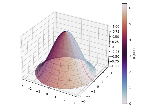
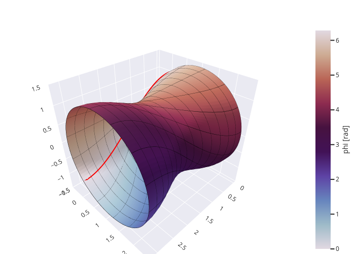
Revolve the same function around an axis parallel to the x axis, using Plotly:
from sympy import symbols, cos, sin, pi
from spb import *
t, phi = symbols('t phi')
graphics(
    surface_revolution(
        cos(t), (t, 0, pi), parallel_axis="x", axis=(1, 0),
        label="phi [rad]", rendering_kw={"colorscale": "twilight"},
        use_cm=True, color_func=lambda t, phi: phi,
        show_curve=True,
        curve_kw=dict(rendering_kw={"line": {"color": "red", "width": 8},
            "name": "cos(t)"}),
        wireframe=True, wf_n1=15, wf_n2=15,
        wf_rendering_kw={"line_width": 1}
    ),
    backend=PB
)
(Source code, png)
Revolve a 2D parametric circle around the z axis:
from sympy import *
from spb import *
t = symbols("t")
circle = (3 + cos(t), sin(t))
graphics(
    surface_revolution(circle, (t, 0, 2 * pi),
        show_curve=True, rendering_kw={"opacity": 0.65},
        curve_kw={"rendering_kw": {"width": 0.05}}),
    backend=KB)

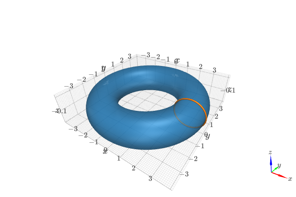
Revolve a 3D parametric curve around the z axis for a given azimuthal angle, using Plotly:
from sympy import *
from spb import *
t = symbols("t")
graphics(
    surface_revolution(
        (cos(t), sin(t), t), (t, 0, 2*pi), (phi, 0, pi),
        use_cm=True, color_func=lambda t, phi: t, label="t [rad]",
        show_curve=True,
        wireframe=True, wf_n1=2, wf_n2=5),
    backend=PB, aspect="cube")
(Source code, png)
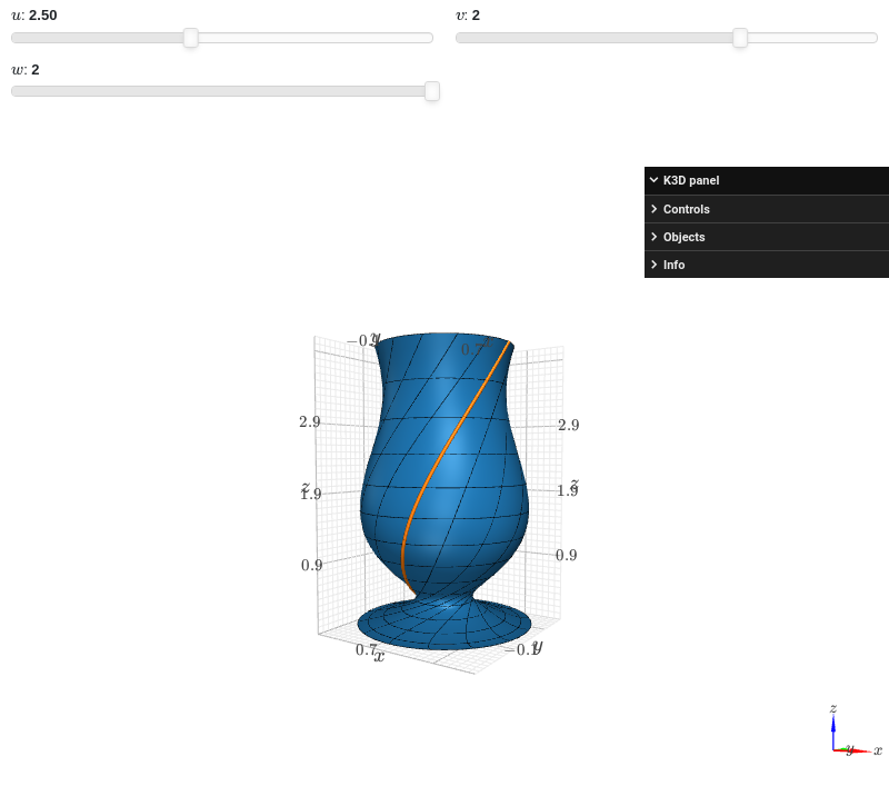
Interactive-widget plot of a goblet. Refer to the interactive sub-module documentation to learn more about the
paramsdictionary. This plot illustrates:the use of
prange(parametric plotting range).the use of the
paramsdictionary to specify sliders in their basic form: (default, min, max).
from sympy import *
from spb import *
t, phi, u, v, w = symbols("t phi u v w")
graphics(
    surface_revolution(
        (t, cos(u * t), t**2), prange(t, 0, v), prange(phi, 0, w*pi),
        axis=(1, 0.2), n=50,
        wireframe=True, wf_n1=15, wf_n2=15,
        wf_rendering_kw={"width": 0.004},
        show_curve=True, curve_kw={"rendering_kw": {"width": 0.025}},
        params={
            u: (2.5, 0, 6),
            v: (2, 0, 3),
            w: (2, 0, 2)
        }),
    backend=KB, force_real_eval=True)

- spb.graphics.functions_3d.surface_spherical(r, range_theta=None, range_phi=None, label=None, rendering_kw=None, **kwargs)[source]
Plots a radius as a function of the spherical coordinates theta and phi.
- Parameters:
- rExpr or callable
Expression representing the radius. It can be a:
Symbolic expression.
Numerical function of two variable, f(theta, phi), supporting vectorization. In this case the following keyword arguments are not supported:
params.
- range_thetatuple
A 3-tuple (symbol, min, max) denoting the range of the polar angle, which is limited in [0, pi]. Consider a sphere:
theta=0indicates the north pole.theta=pi/2indicates the equator.theta=piindicates the south pole.
- range_phituple
A 3-tuple (symbol, min, max) denoting the range of the azimuthal angle, which is limited in [0, 2*pi].
- labelstr
Set the label associated to this series, which will be eventually shown on the legend or colorbar.
- rendering_kwdict
A dictionary of keyword arguments to be passed to the renderers in order to further customize the appearance of the surface. Here are some useful links for the supported plotting libraries:
K3D-Jupyter: look at the documentation of k3d.mesh.
- color_func
Define the surface color mapping when use_cm=True. It can either be:
None: the default value (color mapping according to the z coordinate).
A numerical function supporting vectorization. The arity can be:
1 argument:
f(u), whereuis the first parameter.2 arguments:
f(u, v)whereu, vare the parameters.3 arguments:
f(x, y, z)wherex, y, zare the coordinates of the points.5 arguments:
f(x, y, z, u, v).
A symbolic expression having at most as many free symbols as
expr_xorexpr_yorexpr_z.
- colorbarbool
Toggle the visibility of the colorbar associated to the current data series. Note that a colorbar is only visible if
use_cm=Trueandcolor_funcis not None. Default value: True.- colorbar_ticks_formattertick_formatter_multiples_of
An object of type
tick_formatter_multiples_ofwhich will be used to place tick values on the colorbar at each multiple of a specified quantity. This only works when use_cm=True.- force_real_evalbool
By default, numerical evaluation is performed over complex numbers, which is slower but produces correct results. However, when the symbolic expression is converted to a numerical function with lambdify, the resulting function may not like to be evaluated over complex numbers. In such cases, forcing the evaluation to be performed over real numbers might be a good choice. The plotting module should be able to detect such occurences and automatically activate this option. If that is not the case, or evaluation performance is of paramount importance, set this parameter to True, but be aware that it might produce wrong results. Default value: False.
- modules
Specify the evaluation modules to be used by lambdify. If not specified, the evaluation will be done with NumPy/SciPy.
- n1int
Number of discretization points along the first parameter to be used in the evaluation. Related parameters:
xscale. It must be: 2 ≤ n1 < ∞. Default value: 100.- n2int
Number of discretization points along the second parameter to be used in the evaluation. Related parameters:
yscale. It must be: 2 ≤ n2 < ∞. Default value: 100.- only_integersbool
Discretize the domain using only integer numbers. When this parameter is True, the number of discretization points is choosen by the algorithm. Default value: False.
- paramsdict, optional
A dictionary mapping symbols to parameters. If provided, this dictionary enables the interactive-widgets plot.
When calling a plotting function, the parameter can be specified with:
a widget from the
ipywidgetsmodule.a widget from the
panelmodule.- a tuple of the form:
(default, min, max, N, tick_format, label, spacing), which will instantiate a
ipywidgets.widgets.widget_float.FloatSlideror aipywidgets.widgets.widget_float.FloatLogSlider, depending on the spacing strategy. In particular:- default, min, maxfloat
Default value, minimum value and maximum value of the slider, respectively. Must be finite numbers. The order of these 3 numbers is not important: the module will figure it out which is what.
- Nint, optional
Number of steps of the slider.
- tick_formatstr or None, optional
Provide a formatter for the tick value of the slider. Default to
".2f".
- label: str, optional
Custom text associated to the slider.
- spacingstr, optional
Specify the discretization spacing. Default to
"linear", can be changed to"log".
Notes:
parameters cannot be linked together (ie, one parameter cannot depend on another one).
If a widget returns multiple numerical values (like
panel.widgets.slider.RangeSlideroripywidgets.widgets.widget_float.FloatRangeSlider), then a corresponding number of symbols must be provided.
Here follows a couple of examples. If
imodule="panel":import panel as pn params = { a: (1, 0, 5), # slider from 0 to 5, with default value of 1 b: pn.widgets.FloatSlider(value=1, start=0, end=5), # same slider as above (c, d): pn.widgets.RangeSlider(value=(-1, 1), start=-3, end=3, step=0.1) }
Or with
imodule="ipywidgets":import ipywidgets as w params = { a: (1, 0, 5), # slider from 0 to 5, with default value of 1 b: w.FloatSlider(value=1, min=0, max=5), # same slider as above (c, d): w.FloatRangeSlider(value=(-1, 1), min=-3, max=3, step=0.1) }
When instantiating a data series directly,
paramsmust be a dictionary mapping symbols to numerical values.Let
seriesbe any data series. Thenseries.paramsreturns a dictionary mapping symbols to numerical values.- show_in_legendbool
Toggle the visibility of the data series on the legend. Default value: True.
- sum_boundint
When plotting sums, the expression will be pre-processed in order to replace lower/upper bounds set to +/- infinity with this +/- numerical value. Note: the higher this number, the slower the evaluation, but the more accurate the plot. It must be: 0 ≤ sum_bound < ∞. Default value: 1000.
- surface_color
For back-compatibility with old sympy.plotting. Use
rendering_kwin order to fully customize the appearance of the surface.- txcallable
Numerical transformation function to be applied to the data on the x-axis.
- tycallable
Numerical transformation function to be applied to the data on the y-axis.
- tzcallable
Numerical transformation function to be applied to the data on the z-axis.
- use_cmbool
Toggle the use of a colormap. By default, some series might use a colormap to display the necessary data. Setting this attribute to False will inform the associated renderer to use solid color. Related parameters:
color_func. Default value: False.- xscalestr
Discretization strategy along the first parameter. Related parameters:
n1. Possible options: [‘linear’, ‘log’] Default value: ‘linear’.- yscalestr
Discretization strategy along the second parameter. Related parameters:
n2. Possible options: [‘linear’, ‘log’] Default value: ‘linear’.
- Returns:
- serieslist
A list containing one instance of
ParametricSurfaceSeriesand possibly multiple instances ofParametric3DLineSeries, ifwireframe=True.
See also
Examples
>>> from sympy import symbols, cos, sin, pi, Ynm, re, lambdify
>>> from spb import *
>>> theta, phi = symbols('theta phi')
Sphere cap:
>>> graphics(
...     surface_spherical(1, (theta, 0, 0.7 * pi), (phi, 0, 1.8 * pi)))
Plot object containing:
[0]: parametric cartesian surface: (sin(theta)*cos(phi), sin(phi)*sin(theta), cos(theta)) for theta over (0, 0.7*pi) and phi over (0, 1.8*pi)
(
Source code,png)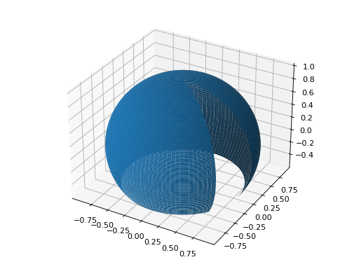
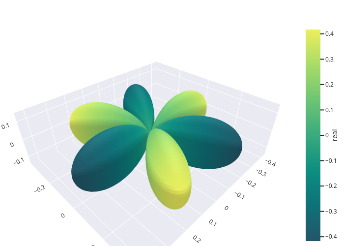
Plot real spherical harmonics, highlighting the regions in which the real part is positive and negative, using Plotly:
from sympy import symbols, sin, pi, Ynm, re, lambdify
from spb import *
theta, phi = symbols('theta phi')
r = re(Ynm(3, 3, theta, phi).expand(func=True).rewrite(sin).expand())
graphics(
    surface_spherical(
        abs(r), (theta, 0, pi), (phi, 0, 2 * pi), "real",
        use_cm=True, n2=200,
        color_func=lambdify([theta, phi], r)),
    backend=PB)
(Source code, png)
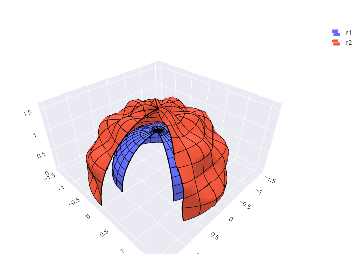
Multiple surfaces with wireframe lines, using Plotly. Note that activating the wireframe option might add a considerable overhead during the plot’s creation.
from sympy import symbols, sin, pi
from spb import *
theta, phi = symbols('theta phi')
r1 = 1
r2 = 1.5 + sin(5 * phi) * sin(10 * theta) / 10
graphics(
    surface_spherical(r1, (theta, 0, pi / 2), (phi, 0.35 * pi, 2 * pi),
        label="r1", wireframe=True, wf_n2=25),
    surface_spherical(r2, (theta, 0, pi / 2), (phi, 0.35 * pi, 2 * pi),
        label="r2", wireframe=True, wf_n2=25),
    backend=PB)
(Source code, png)
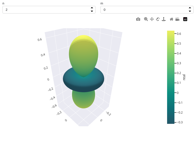
Interactive-widget plot of real spherical harmonics, highlighting the regions in which the real part is positive and negative. Note that the plot’s creation and update might be slow and that it must be
m < nat all times. Refer to the interactive sub-module documentation to learn more about theparamsdictionary.from sympy import * from spb import * import panel as pn n, m = symbols("n, m") phi, theta = symbols("phi, theta", real=True) r = re(Ynm(n, m, theta, phi).expand(func=True).rewrite(sin).expand()) graphics( surface_spherical(abs(r), (theta, 0, pi), (phi, 0, 2*pi), label="real", params = { n: pn.widgets.IntInput(value=2, name="n"), m: pn.widgets.IntInput(value=0, name="m"), }, use_cm=True, color_func=r, force_real_eval=True), backend=PB, imodule="panel")
- spb.graphics.functions_3d.plane(p, range_x=None, range_y=None, range_z=None, label=None, rendering_kw=None, **kwargs)[source]
Plot a plane in a 3D space.
- Parameters:
- pPlane
The plane to be plotted.
- range_xtuple, Tuple
A 3-tuple (symb, min, max) denoting the range of the x variable. Default values: min=-10 and max=10.
- range_ytuple, Tuple
A 3-tuple (symb, min, max) denoting the range of the y variable. Default values: min=-10 and max=10.
- range_ztuple, Tuple
A 3-tuple (symb, min, max) denoting the range of the z variable. Default values: min=-10 and max=10.
- labelstr
Set the label associated to this series, which will be eventually shown on the legend or colorbar.
- rendering_kwdict
A dictionary of keyword arguments to be passed to the renderers in order to further customize the appearance of the surface. Here are some useful links for the supported plotting libraries:
K3D-Jupyter: look at the documentation of k3d.mesh.
- color_func
A color function to be applied to the numerical data. It can be:
None: no color function.
callable: a function of 3 arguments (the coordinates x, y, z) returning numerical data.
- colorbarbool
Toggle the visibility of the colorbar associated to the current data series. Note that a colorbar is only visible if
use_cm=Trueandcolor_funcis not None. Default value: True.- colorbar_ticks_formattertick_formatter_multiples_of
An object of type
tick_formatter_multiples_ofwhich will be used to place tick values on the colorbar at each multiple of a specified quantity. This only works when use_cm=True.- force_real_evalbool
By default, numerical evaluation is performed over complex numbers, which is slower but produces correct results. However, when the symbolic expression is converted to a numerical function with lambdify, the resulting function may not like to be evaluated over complex numbers. In such cases, forcing the evaluation to be performed over real numbers might be a good choice. The plotting module should be able to detect such occurences and automatically activate this option. If that is not the case, or evaluation performance is of paramount importance, set this parameter to True, but be aware that it might produce wrong results. Default value: False.
- modules
Specify the evaluation modules to be used by lambdify. If not specified, the evaluation will be done with NumPy/SciPy.
- n1int
Number of discretization points along the x-axis to be used in the evaluation. Related parameters:
xscale. It must be: 2 ≤ n1 < ∞. Default value: 20.- n2int
Number of discretization points along the y-axis to be used in the evaluation. Related parameters:
yscale. It must be: 2 ≤ n2 < ∞. Default value: 20.- n3int
Number of discretization points along the z-axis to be used in the evaluation. Related parameters:
zscale. It must be: 2 ≤ n3 < ∞. Default value: 20.- only_integersbool
Discretize the domain using only integer numbers. When this parameter is True, the number of discretization points is choosen by the algorithm. Default value: False.
- paramsdict, optional
A dictionary mapping symbols to parameters. If provided, this dictionary enables the interactive-widgets plot.
When calling a plotting function, the parameter can be specified with:
a widget from the
ipywidgetsmodule.a widget from the
panelmodule.- a tuple of the form:
(default, min, max, N, tick_format, label, spacing), which will instantiate a
ipywidgets.widgets.widget_float.FloatSlideror aipywidgets.widgets.widget_float.FloatLogSlider, depending on the spacing strategy. In particular:- default, min, maxfloat
Default value, minimum value and maximum value of the slider, respectively. Must be finite numbers. The order of these 3 numbers is not important: the module will figure it out which is what.
- Nint, optional
Number of steps of the slider.
- tick_formatstr or None, optional
Provide a formatter for the tick value of the slider. Default to
".2f".
- label: str, optional
Custom text associated to the slider.
- spacingstr, optional
Specify the discretization spacing. Default to
"linear", can be changed to"log".
Notes:
parameters cannot be linked together (ie, one parameter cannot depend on another one).
If a widget returns multiple numerical values (like
panel.widgets.slider.RangeSlideroripywidgets.widgets.widget_float.FloatRangeSlider), then a corresponding number of symbols must be provided.
Here follows a couple of examples. If
imodule="panel":import panel as pn params = { a: (1, 0, 5), # slider from 0 to 5, with default value of 1 b: pn.widgets.FloatSlider(value=1, start=0, end=5), # same slider as above (c, d): pn.widgets.RangeSlider(value=(-1, 1), start=-3, end=3, step=0.1) }
Or with
imodule="ipywidgets":import ipywidgets as w params = { a: (1, 0, 5), # slider from 0 to 5, with default value of 1 b: w.FloatSlider(value=1, min=0, max=5), # same slider as above (c, d): w.FloatRangeSlider(value=(-1, 1), min=-3, max=3, step=0.1) }
When instantiating a data series directly,
paramsmust be a dictionary mapping symbols to numerical values.Let
seriesbe any data series. Thenseries.paramsreturns a dictionary mapping symbols to numerical values.- show_in_legendbool
Toggle the visibility of the data series on the legend. Default value: True.
- sum_boundint
When plotting sums, the expression will be pre-processed in order to replace lower/upper bounds set to +/- infinity with this +/- numerical value. Note: the higher this number, the slower the evaluation, but the more accurate the plot. It must be: 0 ≤ sum_bound < ∞. Default value: 1000.
- surface_color
For back-compatibility with old sympy.plotting. Use
rendering_kwin order to fully customize the appearance of the surface.- txcallable
Numerical transformation function to be applied to the data on the x-axis.
- tycallable
Numerical transformation function to be applied to the data on the y-axis.
- tzcallable
Numerical transformation function to be applied to the data on the z-axis.
- use_cmbool
Toggle the use of a colormap. By default, some series might use a colormap to display the necessary data. Setting this attribute to False will inform the associated renderer to use solid color. Related parameters:
color_func. Default value: False.- xscalestr
Discretization strategy along the x-direction. Related parameters:
n1. Possible options: [‘linear’, ‘log’] Default value: ‘linear’.- yscalestr
Discretization strategy along the y-direction. Related parameters:
n2. Possible options: [‘linear’, ‘log’] Default value: ‘linear’.- zscalestr
Discretization strategy along the z-direction. Related parameters:
n3. Possible options: [‘linear’, ‘log’] Default value: ‘linear’.
- Returns:
- serieslist
A list containing an instance of
PlaneSeries.
See also
Examples
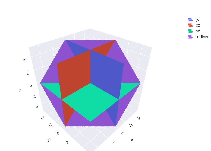
from sympy import *
from spb import *
from sympy.abc import x, y, z
ranges = [(x, -5, 5), (y, -5, 5), (z, -5, 5)]
graphics(
    plane(Plane((0, 0, 0), (1, 0, 0)), *ranges, label="yz"),
    plane(Plane((0, 0, 0), (0, 1, 0)), *ranges, label="xz"),
    plane(Plane((0, 0, 0), (0, 0, 1)), *ranges, label="yz"),
    plane(Plane((0, 0, 0), (1, 1, 1)), *ranges, label="inclined", n=150),
    backend=PB, xlabel="x", ylabel="y", zlabel="z"
)
(Source code, png)
- spb.graphics.functions_3d.implicit_3d(expr, range_x=None, range_y=None, range_z=None, label=None, rendering_kw=None, **kwargs)[source]
Plots an isosurface or a volumetric plot of a function.
- Parameters:
- expr
Implicit expression. It can be a:
Symbolic expression.
- Numerical function of three variable, f(x, y, z), supporting
vectorization.
- range_xtuple, Tuple
A 3-tuple (symb, min, max) denoting the range of the x variable. Default values: min=-10 and max=10.
- range_ytuple, Tuple
A 3-tuple (symb, min, max) denoting the range of the y variable. Default values: min=-10 and max=10.
- range_ztuple, Tuple
A 3-tuple (symb, min, max) denoting the range of the z variable. Default values: min=-10 and max=10.
- labelstr
Set the label associated to this series, which will be eventually shown on the legend or colorbar.
- rendering_kwdict
A dictionary of keyword arguments to be passed to the renderers in order to further customize the appearance of the surface. Here are some useful links for the supported plotting libraries:
K3D-Jupyter: look at the documentation of k3d.marching_cubes.
- colorbarbool
Toggle the visibility of the colorbar associated to the current data series. Note that a colorbar is only visible if
use_cm=Trueandcolor_funcis not None. Default value: True.- colorbar_ticks_formattertick_formatter_multiples_of
An object of type
tick_formatter_multiples_ofwhich will be used to place tick values on the colorbar at each multiple of a specified quantity. This only works when use_cm=True.- force_real_evalbool
By default, numerical evaluation is performed over complex numbers, which is slower but produces correct results. However, when the symbolic expression is converted to a numerical function with lambdify, the resulting function may not like to be evaluated over complex numbers. In such cases, forcing the evaluation to be performed over real numbers might be a good choice. The plotting module should be able to detect such occurences and automatically activate this option. If that is not the case, or evaluation performance is of paramount importance, set this parameter to True, but be aware that it might produce wrong results. Default value: False.
- modules
Specify the evaluation modules to be used by lambdify. If not specified, the evaluation will be done with NumPy/SciPy.
- n1int
Number of discretization points along the x-axis to be used in the evaluation. Related parameters:
xscale. It must be: 2 ≤ n1 < ∞. Default value: 60.- n2int
Number of discretization points along the y-axis to be used in the evaluation. Related parameters:
yscale. It must be: 2 ≤ n2 < ∞. Default value: 60.- n3int
Number of discretization points along the z-axis to be used in the evaluation. Related parameters:
zscale. It must be: 2 ≤ n3 < ∞. Default value: 60.- only_integersbool
Discretize the domain using only integer numbers. When this parameter is True, the number of discretization points is choosen by the algorithm. Default value: False.
- paramsdict, optional
A dictionary mapping symbols to parameters. If provided, this dictionary enables the interactive-widgets plot.
When calling a plotting function, the parameter can be specified with:
a widget from the
ipywidgetsmodule.a widget from the
panelmodule.- a tuple of the form:
(default, min, max, N, tick_format, label, spacing), which will instantiate a
ipywidgets.widgets.widget_float.FloatSlideror aipywidgets.widgets.widget_float.FloatLogSlider, depending on the spacing strategy. In particular:- default, min, maxfloat
Default value, minimum value and maximum value of the slider, respectively. Must be finite numbers. The order of these 3 numbers is not important: the module will figure it out which is what.
- Nint, optional
Number of steps of the slider.
- tick_formatstr or None, optional
Provide a formatter for the tick value of the slider. Default to
".2f".
- label: str, optional
Custom text associated to the slider.
- spacingstr, optional
Specify the discretization spacing. Default to
"linear", can be changed to"log".
Notes:
parameters cannot be linked together (ie, one parameter cannot depend on another one).
If a widget returns multiple numerical values (like
panel.widgets.slider.RangeSlideroripywidgets.widgets.widget_float.FloatRangeSlider), then a corresponding number of symbols must be provided.
Here follows a couple of examples. If
imodule="panel":import panel as pn params = { a: (1, 0, 5), # slider from 0 to 5, with default value of 1 b: pn.widgets.FloatSlider(value=1, start=0, end=5), # same slider as above (c, d): pn.widgets.RangeSlider(value=(-1, 1), start=-3, end=3, step=0.1) }
Or with
imodule="ipywidgets":import ipywidgets as w params = { a: (1, 0, 5), # slider from 0 to 5, with default value of 1 b: w.FloatSlider(value=1, min=0, max=5), # same slider as above (c, d): w.FloatRangeSlider(value=(-1, 1), min=-3, max=3, step=0.1) }
When instantiating a data series directly,
paramsmust be a dictionary mapping symbols to numerical values.Let
seriesbe any data series. Thenseries.paramsreturns a dictionary mapping symbols to numerical values.- show_in_legendbool
Toggle the visibility of the data series on the legend. Default value: True.
- sum_boundint
When plotting sums, the expression will be pre-processed in order to replace lower/upper bounds set to +/- infinity with this +/- numerical value. Note: the higher this number, the slower the evaluation, but the more accurate the plot. It must be: 0 ≤ sum_bound < ∞. Default value: 1000.
- surface_color
For back-compatibility with old sympy.plotting. Use
rendering_kwin order to fully customize the appearance of the surface.- txcallable
Numerical transformation function to be applied to the data on the x-axis.
- tycallable
Numerical transformation function to be applied to the data on the y-axis.
- tzcallable
Numerical transformation function to be applied to the data on the z-axis.
- use_cmbool
Toggle the use of a colormap. By default, some series might use a colormap to display the necessary data. Setting this attribute to False will inform the associated renderer to use solid color. Related parameters:
color_func. Default value: False.- xscalestr
Discretization strategy along the x-direction. Related parameters:
n1. Possible options: [‘linear’, ‘log’] Default value: ‘linear’.- yscalestr
Discretization strategy along the y-direction. Related parameters:
n2. Possible options: [‘linear’, ‘log’] Default value: ‘linear’.- zscalestr
Discretization strategy along the z-direction. Related parameters:
n3. Possible options: [‘linear’, ‘log’] Default value: ‘linear’.
- Returns:
- serieslist
A list containing one instance of
Implicit3DSeries.
See also
Notes
the number of discretization points is crucial as the algorithm will discretize a volume. A high number of discretization points creates a smoother mesh, at the cost of a much higher memory consumption and slower computation.
Only
PlotlyBackendandK3DBackendsupport 3D implicit plotting.To plot
f(x, y, z) = ceither writeexpr = f(x, y, z) - cor pass the appropriate keyword torendering_kw. Read the backends documentation to find out the available options.Volumetric plots will use voxels.
Examples
from sympy import symbols
from spb import *
x, y, z = symbols('x, y, z')
graphics(
    implicit_3d(x**2 + y**3 - z**2, (x, -2, 2), (y, -2, 2), (z, -2, 2)),
    backend=PB)
(Source code, png)
graphics(
    implicit_3d(x**4 + y**4 + z**4 - (x**2 + y**2 + z**2 - 0.3),
        (x, -2, 2), (y, -2, 2), (z, -2, 2)),
    backend=PB)
(Source code, png)
Visualize the isocontours from isomin=0 to isomax=2 by providing a
rendering_kwdictionary:graphics( implicit_3d(1/x**2 - 1/y**2 + 1/z**2, (x, -2, 2), (y, -2, 2), (z, -2, 2), rendering_kw={ "isomin": 0, "isomax": 2, "colorscale":"aggrnyl", "showscale":True }), backend=PB )
(Source code, png)
Volumetric plots:
from sympy import *
from spb import *
var("x:z")
graphics(
    implicit_3d(x*y*z < 1, (x, -5, 5), (y, -5, 5), (z, -5, 5), n=150),
    backend=KB
)
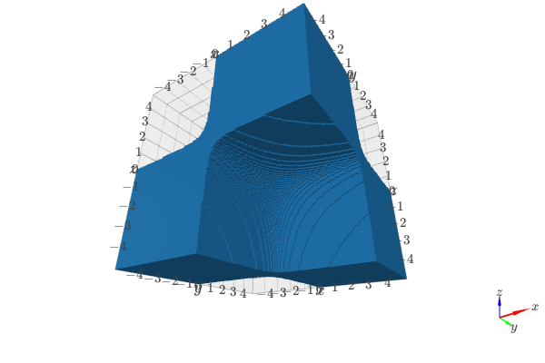
from sympy import *
from spb import *
var("x:z")
graphics(
    implicit_3d(
        (x**2 + y**2 + z**2 >= 1) & (x**2 + y**2 + z**2 <= 3) & (y >= 0),
        (x, -2, 2), (y, -2, 2), (z, -2, 2), n=150),
    backend=KB
)
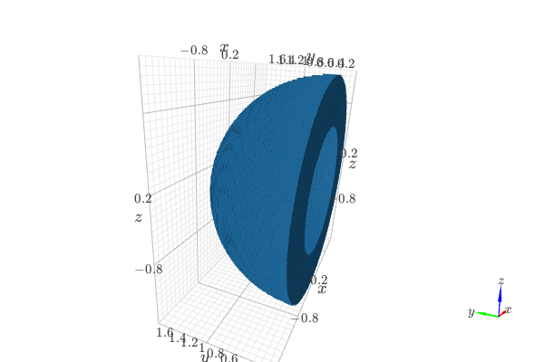
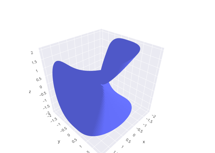
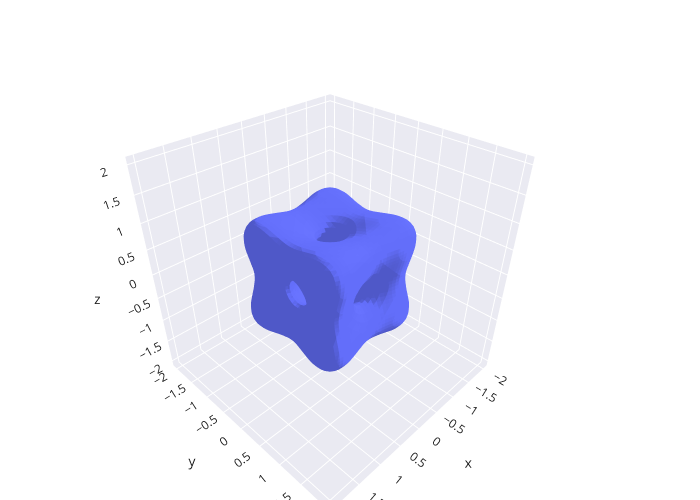
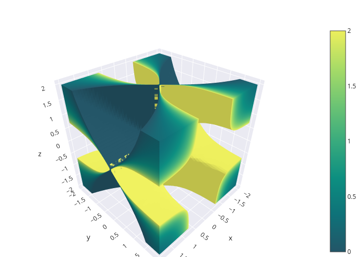
- spb.graphics.functions_3d.wireframe(surface_series, n1=10, n2=10, n=None, rendering_kw=None, **kwargs)[source]
Creates a wireframe of a 3D surface.
- Parameters:
- surface_seriesBaseSeries
A data series representing a surface.
- n1int, optional
Number of wireframe lines along the first direction (or range).
- n2int, optional
Number of wireframe lines along the second direction (or range).
- nint, optional
Number of evaluation points for each wireframe line. If not provided, the algorithm will chose the number of discretization points from the
surface_series. The higher this number, the slower the creation of the plot.- rendering_kwdict
A dictionary of keyword arguments to be passed to the renderers in order to further customize the appearance of the line. Here are some useful links for the supported plotting libraries:
Matplotlib:
for solid lines: https://matplotlib.org/stable/api/_as_gen/matplotlib.pyplot.plot.html
for colormap-based lines: https://matplotlib.org/stable/api/collections_api.html#matplotlib.collections.LineCollection
for scatters: https://matplotlib.org/stable/api/_as_gen/matplotlib.pyplot.scatter.html
Bokeh:
- color_func
Define a custom color mapping when
use_cm=True. It can either be:A numerical function supporting vectorization. The arity can be:
1 argument:
f(t), wheretis the parameter.3 arguments:
f(x, y, z)wherex, y, zare the coordinates of the points.4 arguments:
f(x, y, z, t).
A symbolic expression having at most as many free symbols as
expr_xorexpr_yorexpr_z.None: the default value (color mapping according to the parameter).
Alias of this parameters:
tp.- colorbarbool
Toggle the visibility of the colorbar associated to the current data series. Note that a colorbar is only visible if
use_cm=Trueandcolor_funcis not None. Default value: True.- colorbar_ticks_formattertick_formatter_multiples_of
An object of type
tick_formatter_multiples_ofwhich will be used to place tick values on the colorbar at each multiple of a specified quantity. This only works when use_cm=True.- detect_polesbool, str
Chose whether to detect and correctly plot the roots of the denominator. There are two algorithms at work:
based on the gradient of the numerical data, it introduces NaN values at locations where the steepness is greater than some threshold. This splits the line into multiple segments. To improve detection, increase the number of discretization points
nand/or change the value ofeps. This algorithm can be used to visualize jump discontinuities as well as essential discontinuities.a symbolic approach based on the
continuous_domainfunction from thesympy.calculus.utilmodule, which computes the locations of essential discontinuities. If any are found, vertical lines will be shown.
Possible options:
False: No poles detection
True: Poles detection with the numerical algorithm
‘symbolic’: Poles detection with numerical and symbolic algorithms
Default value: False.
- epsfloat
An arbitrary small value used by the
detect_polesnumerical algorithm. Before changing this value, it is recommended to increase the number of discretization points. Related parameters:detect_poles. It must be: 0 ≤ eps < ∞. Default value: 0.01.- excludelist
A list of numerical values along the parameter which are going to be excluded from the evaluation. In practice, it introduces discontinuities in the resulting line.
- force_real_evalbool
By default, numerical evaluation is performed over complex numbers, which is slower but produces correct results. However, when the symbolic expression is converted to a numerical function with lambdify, the resulting function may not like to be evaluated over complex numbers. In such cases, forcing the evaluation to be performed over real numbers might be a good choice. The plotting module should be able to detect such occurences and automatically activate this option. If that is not the case, or evaluation performance is of paramount importance, set this parameter to True, but be aware that it might produce wrong results. Default value: False.
- is_filledbool
Whether scatter’s markers are filled or void. Default value: True.
- is_scatterbool
If True it represent a scatter plot, otherwise a continuous line. Default value: False.
- labelstr
Set the label associated to this series, which will be eventually shown on the legend or colorbar.
- line_color
For back-compatibility with old sympy.plotting. Use
rendering_kwin order to fully customize the appearance of the line/scatter.- modules
Specify the evaluation modules to be used by lambdify. If not specified, the evaluation will be done with NumPy/SciPy.
- only_integersbool
Discretize the domain using only integer numbers. When this parameter is True, the number of discretization points is choosen by the algorithm. Default value: False.
- paramsdict, optional
A dictionary mapping symbols to parameters. If provided, this dictionary enables the interactive-widgets plot.
When calling a plotting function, the parameter can be specified with:
a widget from the
ipywidgetsmodule.a widget from the
panelmodule.- a tuple of the form:
(default, min, max, N, tick_format, label, spacing), which will instantiate a
ipywidgets.widgets.widget_float.FloatSlideror aipywidgets.widgets.widget_float.FloatLogSlider, depending on the spacing strategy. In particular:- default, min, maxfloat
Default value, minimum value and maximum value of the slider, respectively. Must be finite numbers. The order of these 3 numbers is not important: the module will figure it out which is what.
- Nint, optional
Number of steps of the slider.
- tick_formatstr or None, optional
Provide a formatter for the tick value of the slider. Default to
".2f".
- label: str, optional
Custom text associated to the slider.
- spacingstr, optional
Specify the discretization spacing. Default to
"linear", can be changed to"log".
Notes:
parameters cannot be linked together (ie, one parameter cannot depend on another one).
If a widget returns multiple numerical values (like
panel.widgets.slider.RangeSlideroripywidgets.widgets.widget_float.FloatRangeSlider), then a corresponding number of symbols must be provided.
Here follows a couple of examples. If
imodule="panel":import panel as pn params = { a: (1, 0, 5), # slider from 0 to 5, with default value of 1 b: pn.widgets.FloatSlider(value=1, start=0, end=5), # same slider as above (c, d): pn.widgets.RangeSlider(value=(-1, 1), start=-3, end=3, step=0.1) }
Or with
imodule="ipywidgets":import ipywidgets as w params = { a: (1, 0, 5), # slider from 0 to 5, with default value of 1 b: w.FloatSlider(value=1, min=0, max=5), # same slider as above (c, d): w.FloatRangeSlider(value=(-1, 1), min=-3, max=3, step=0.1) }
When instantiating a data series directly,
paramsmust be a dictionary mapping symbols to numerical values.Let
seriesbe any data series. Thenseries.paramsreturns a dictionary mapping symbols to numerical values.- show_in_legendbool
Toggle the visibility of the data series on the legend. Default value: True.
- sum_boundint
When plotting sums, the expression will be pre-processed in order to replace lower/upper bounds set to +/- infinity with this +/- numerical value. Note: the higher this number, the slower the evaluation, but the more accurate the plot. It must be: 0 ≤ sum_bound < ∞. Default value: 1000.
- txcallable
Numerical transformation function to be applied to the data on the x-axis.
- tycallable
Numerical transformation function to be applied to the data on the y-axis.
- tzcallable
Numerical transformation function to be applied to the data on the z-axis.
- use_cmbool
Toggle the use of a colormap. By default, some series might use a colormap to display the necessary data. Setting this attribute to False will inform the associated renderer to use solid color. Related parameters:
color_func. Default value: False.- xscalestr
Discretization strategy along the parameter. Possible options: [‘linear’, ‘log’] Default value: ‘linear’.
- Returns:
- serieslist
A list containing instances of
Parametric3DLineSeries.
See also
Examples
Provide better code separation between the surface and wireframe:
from sympy import *
from spb import *
import numpy as np
x, y = symbols("x y")
surf_series = surface(
    cos(x*y) * exp(-sqrt(x**2 + y**2) / 4), (x, -pi, pi), (y, -pi, pi),
    use_cm=True, color_func=lambda x, y, z: np.sqrt(x**2 + y**2)
)
graphics(
    surf_series,
    wireframe(surf_series[0], n1=11, n2=11),
    backend=PB, aspect=dict(x=1.5, y=1.5, z=1)
)
(Source code, png)
Show wireframe without showing the actual surface. Here, dotted wireframe represent the half-unit sphere.
from sympy import *
from spb import *
var("t u v theta phi")
r_sphere = 1
sphere = surface_spherical(1, (theta, 0, pi), (phi, pi, 2*pi))[0]
t = pi / 3 # half-cone angle
r_cone = r_sphere * sin(t)
graphics(
    wireframe(sphere, n1=13, rendering_kw={"line_dash": "dot"}),
    surface_spherical(1, (theta, pi - t, pi), (phi, pi, 2*pi),
        label="sphere cap", wireframe=True, wf_n1=5),
    surface_parametric(
        u * cos(v), u * sin(v), -u / tan(t), (u, 0, r_cone), (v, pi , 2*pi),
        label="cone", wireframe=True, wf_n1=7),
    backend=PB, grid=False
)
(Source code, png)
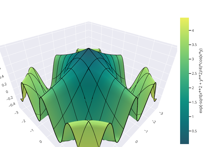
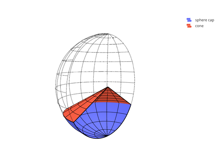