Control

This module contains plotting functions for some of the common plots used in control system. It works with transfer functions from SymPy, SciPy and the control module. To achieve this seamlessly user experience, the control module must be installed, which solves some critical issues related to SymPy but also comes with it’s own quirks.

In particular, impulse_response, step_response and ramp_response provide two modes of operation:

control=True (default value): the symbolic transfer function is converted to a transfer function of the control module. The responses are computed with numerical integration.
control=False the responses are computed with the inverse Laplace transform of the symbolic output signal. This step is not trivial: sometimes it works fine, other times it produces wrong results, other times it consumes too much memory, potentially crashing the machine.

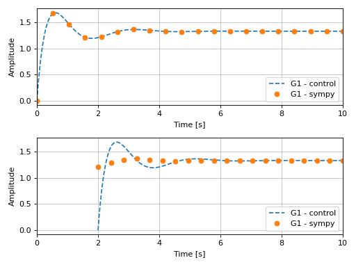
These functions exposes the lower_limit=0 keyword argument, which is the lower value of the time axis. If the default value (zero) is used, the responses from the two modes of operation are identical. On the other hand, if the value is different from zero, then results are different, with the second mode of operation being correct. The first mode of operation is wrong because the integration starts with a zero initial condition.

from sympy import *
from spb import *
x = symbols("x")
s = symbols("s")
G = (8*s**2 + 18*s + 32) / (s**3 + 6*s**2 + 14*s + 24)
p1 = graphics(
   step_response(G, upper_limit=10, label="G1 - control", control=True, rendering_kw={"linestyle": "--"}),
   step_response(G, upper_limit=10, label="G1 - sympy", control=False, scatter=True, n=20),
   xlabel="Time [s]", ylabel="Amplitude", xlim=(0, 10), show=False
)
p2 = graphics(
   step_response(G, upper_limit=10, label="G1 - control", control=True, rendering_kw={"linestyle": "--"}, lower_limit=2),
   step_response(G, upper_limit=10, label="G1 - sympy", control=False, scatter=True, n=20, lower_limit=2),
   xlabel="Time [s]", ylabel="Amplitude", xlim=(0, 10), show=False
)
plotgrid(p1, p2)

(Source code, png)

The plotting module will warn the user if the first mode of operation is being used with a lower_limit different than zero.

NOTES:

All the following examples are generated using Matplotlib. However, Bokeh can be used too, which allows for a better data exploration thanks to useful tooltips. Set backend=BB in the function call to use Bokeh.
For technical reasons, all interactive-widgets plots in this documentation are created using Holoviz’s Panel. Often, they will ran just fine with ipywidgets too. However, if a specific example uses the param library, or widgets from the panel module, then users will have to modify the params dictionary in order to make it work with ipywidgets. Refer to Interactive module for more information.

spb.graphics.control.pole_zero(system, pole_markersize=10, zero_markersize=7, show_axes=False, label=None, sgrid=False, zgrid=False, control=True, input=None, output=None, **kwargs)[source]

Computes the [Pole-Zero] plot (also known as PZ Plot or PZ Map) of a system.

A Pole-Zero plot is a graphical representation of a system’s poles and zeros. It is plotted on a complex plane, with circular markers representing the system’s zeros and ‘x’ shaped markers representing the system’s poles.

Parameters:

systemLTI system type

The system for which the pole-zero plot is to be computed. It can be:

an instance of sympy.physics.control.lti.TransferFunction or sympy.physics.control.lti.TransferFunctionMatrix
an instance of control.TransferFunction
an instance of scipy.signal.TransferFunction
a symbolic expression in rational form, which will be converted to an object of type sympy.physics.control.lti.TransferFunction.
a tuple of two or three elements: (num, den, generator [opt]), which will be converted to an object of type sympy.physics.control.lti.TransferFunction.

pole_colorstr, tuple, optional

The color of the pole points on the plot.

pole_markersizeNumber, optional

The size of the markers used to mark the poles in the plot. Default pole markersize is 10.

zero_colorstr, tuple, optional

The color of the zero points on the plot.

zero_markersizeNumber, optional

The size of the markers used to mark the zeros in the plot. Default zero markersize is 7.

z_rendering_kwdict

A dictionary of keyword arguments to further customize the appearance of zeros.

p_rendering_kwdict

A dictionary of keyword arguments to further customize the appearance of poles.

labelstr, optional

The label to be shown on the legend.

sgridbool, optional

Generates a grid of constant damping ratios and natural frequencies on the s-plane. Default to False.

zgridbool, optional

Generates a grid of constant damping ratios and natural frequencies on the z-plane. Default to False.

controlbool, optional

If True, computes the poles/zeros with the control module, which uses numerical integration. If False, computes them with sympy. Default to True.

inputint, optional

Only compute the poles/zeros for the listed input. If not specified, the poles/zeros for each independent input are computed (as separate traces).

outputint, optional

Only compute the poles/zeros for the listed output. If not specified, all outputs are reported.

**kwargs

See plot for a list of keyword arguments to further customize the resulting figure.

Returns:

A list containing:

one instance of SGridLineSeries if sgrid=True.
one instance of ZGridLineSeries if zgrid=True.
one or more instances of PoleZeroWithSympySeries if control=False.
one or more instances of PoleZeroSeries if control=True.

See also

sgrid, zgrid, root_locus

References

[1]

https://en.wikipedia.org/wiki/Pole%E2%80%93zero_plot

Examples

from sympy.abc import s
from sympy import I
from sympy.physics.control.lti import TransferFunction
from spb import *
tf1 = TransferFunction(
    s**2 + 1, s**4 + 4*s**3 + 6*s**2 + 5*s + 2, s)
graphics(
    pole_zero(tf1, sgrid=True),
    grid=False, xlabel="Real", ylabel="Imaginary"
)

(Source code, png)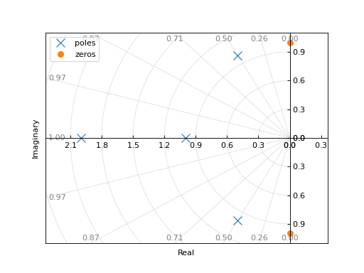

Plotting poles and zeros on the z-plane:

graphics(
    pole_zero(tf1, zgrid=True),
    grid=False, xlabel="Real", ylabel="Imaginary"
)

(Source code, png)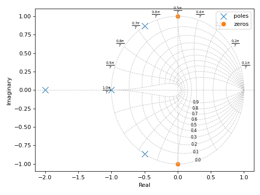

If a transfer function has complex coefficients, make sure to request the evaluation using sympy instead of the control module:

tf = TransferFunction(s + 2, s**2 + (2+I)*s + 10, s)
graphics(
    control_axis(),
    pole_zero(tf, control=False),
    grid=False, xlabel="Real", ylabel="Imaginary"
)

(Source code, png)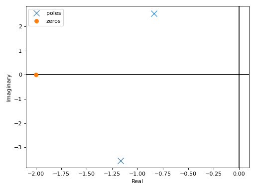

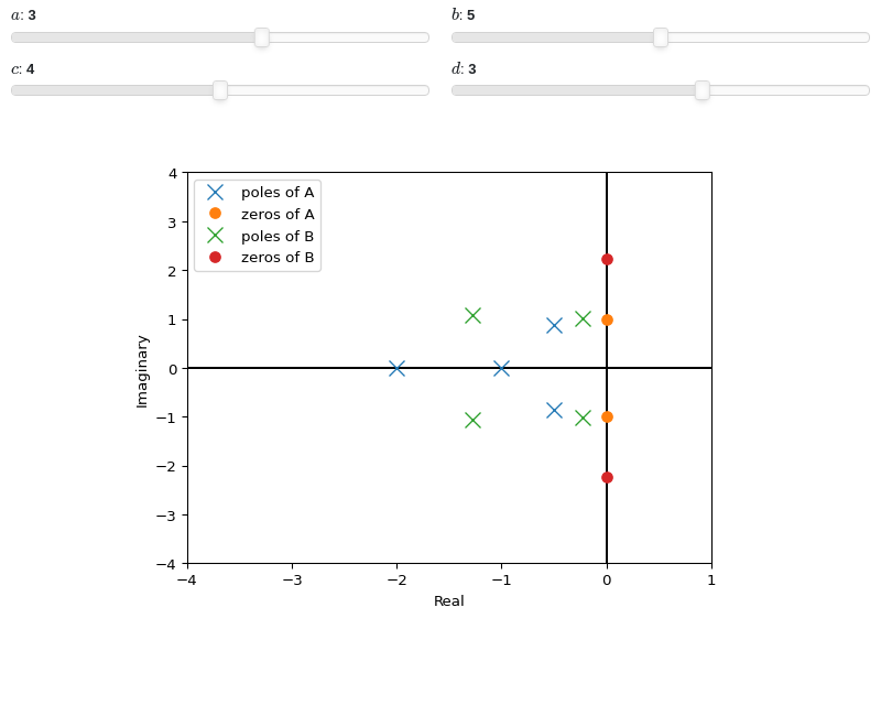
Interactive-widgets plot of multiple systems, one of which is parametric:

from sympy.abc import a, b, c, d, s
from sympy.physics.control.lti import TransferFunction
from spb import *
tf1 = TransferFunction(s**2 + 1, s**4 + 4*s**3 + 6*s**2 + 5*s + 2, s)
tf2 = TransferFunction(s**2 + b, s**4 + a*s**3 + b*s**2 + c*s + d, s)
params = {
    a: (3, 0, 5),
    b: (5, 0, 10),
    c: (4, 0, 8),
    d: (3, 0, 5),
}
graphics(
    control_axis(),
    pole_zero(tf1, label="A"),
    pole_zero(tf2, label="B", params=params),
    grid=False, xlim=(-4, 1), ylim=(-4, 4),
    xlabel="Real", ylabel="Imaginary")

(Source code, small.png)

spb.graphics.control.impulse_response(system, prec=8, lower_limit=None, upper_limit=None, label=None, rendering_kw=None, control=True, input=None, output=None, **kwargs)[source]

Returns the unit impulse response (Input is the Dirac-Delta Function) of a continuous-time system

Parameters:

systemLTI system type

The system for which the impulse response plot is to be computed. It can be:

an instance of sympy.physics.control.lti.TransferFunction or sympy.physics.control.lti.TransferFunctionMatrix
an instance of control.TransferFunction
an instance of scipy.signal.TransferFunction
a symbolic expression in rational form, which will be converted to an object of type sympy.physics.control.lti.TransferFunction.
a tuple of two or three elements: (num, den, generator [opt]), which will be converted to an object of type sympy.physics.control.lti.TransferFunction.

lower_limitNumber or None, optional

The lower time limit of the plot range. Defaults to 0. If a different value is to be used, also set control=False (see examples in order to understand why).

upper_limitNumber or None, optional

The upper time limit of the plot range. If not provided, an appropriate value will be computed. If a interactive widget plot is being created, it defaults to 10.

precint, optional

The decimal point precision for the point coordinate values. Defaults to 8.

labelstr, optional

The label to be shown on the legend.

rendering_kwdict, optional

A dictionary of keywords/values which is passed to the backend’s function to customize the appearance of lines. Refer to the plotting library (backend) manual for more informations.

controlbool, optional

If True, computes the impulse response with the control module, which uses numerical integration. If False, computes the impulse response with sympy, which uses the inverse Laplace transform. Default to True.

control_kwdict, optional

A dictionary of keyword arguments passed to control.impulse_response()

inputint, optional

Only compute the impulse response for the listed input. If not specified, the impulse responses for each independent input are computed (as separate traces).

outputint, optional

Only compute the impulse response for the listed output. If not specified, all outputs are reported.

**kwargs

Keyword arguments are the same as line(). Refer to its documentation for a for a full list of keyword arguments.

Returns:

A list containing one or more instances of:

LineOver1DRangeSeries if control=False.
SystemResponseSeries if control=True.

See also

step_response, ramp_response

References

[1]

https://www.mathworks.com/help/control/ref/lti.impulse.html

Examples

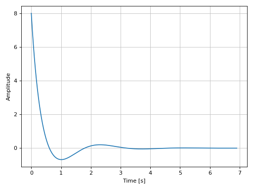
Plotting a SISO system:

from sympy.abc import s
from sympy.physics.control.lti import TransferFunction
from spb import *
tf1 = TransferFunction(
    8*s**2 + 18*s + 32, s**3 + 6*s**2 + 14*s + 24, s)
graphics(
    impulse_response(tf1),
    xlabel="Time [s]", ylabel="Amplitude"
)

(Source code, png)

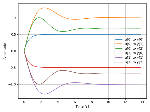
Plotting a MIMO system:

from sympy.physics.control.lti import TransferFunctionMatrix
tf1 = TransferFunction(1, s + 2, s)
tf2 = TransferFunction(s + 1, s**2 + s + 1, s)
tf3 = TransferFunction(s + 1, s**2 + s + 1.5, s)
tfm = TransferFunctionMatrix(
    [[tf1, -tf1], [tf2, -tf2], [tf3, -tf3]])
graphics(
    impulse_response(tfm),
    xlabel="Time [s]", ylabel="Amplitude"
)

(Source code, png)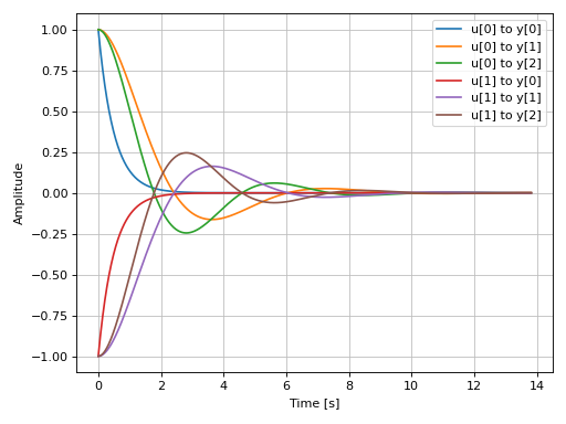

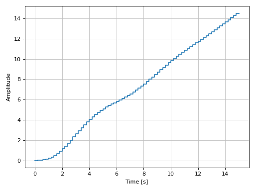
Plotting a discrete-time system:

import control as ct
G = ct.tf([0.0244, 0.0236], [1.1052, -2.0807, 1.0236], dt=0.2)
graphics(
    impulse_response(G, upper_limit=15),
    xlabel="Time [s]", ylabel="Amplitude"
)

(Source code, png)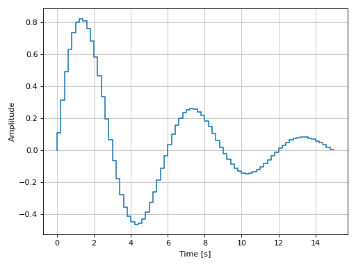

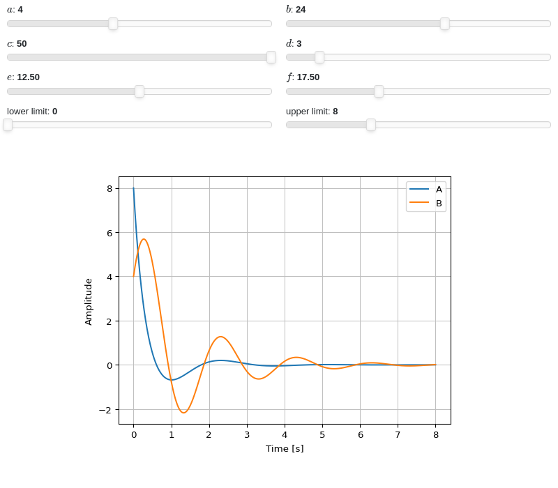
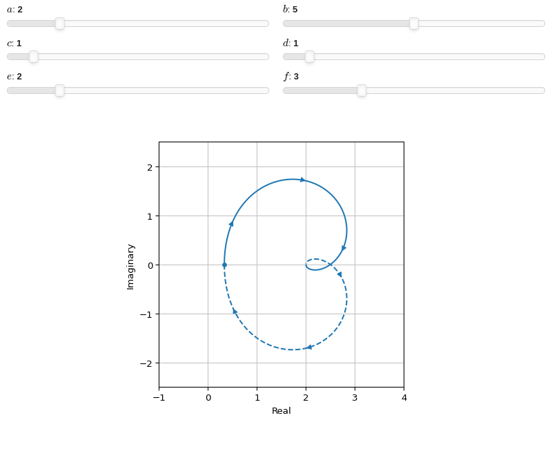
Interactive-widgets plot of multiple systems, one of which is parametric. A few observations:

The first system’s response will be computed with SymPy because control=False was set.
The second system’s response will be computed with the control module, because control=True was set.
Note the use of parametric lower_limit and upper_limit.
By moving the “lower limit” slider, the first system (evaluated with SymPy) will start from some amplitude value. However, on the second system (evaluated with the control module), the amplitude always starts from 0. That’s because the numerical integration’s initial condition is 0. Hence, if lower_limit is to be used, please set control=False.

from sympy.abc import a, b, c, d, e, f, g, h, s
from sympy.physics.control.lti import TransferFunction
from spb import *
tf1 = TransferFunction(8*s**2 + 18*s + 32, s**3 + 6*s**2 + 14*s + 24, s)
tf2 = TransferFunction(a*s**2 + b*s + c, s**3 + d*s**2 + e*s + f, s)
params = {
    a: (4, 0, 10),
    b: (24, 0, 40),
    c: (50, 0, 50),
    d: (3, 0, 25),
    e: (12.5, 0, 25),
    f: (17.5, 0, 50),
    g: (0, 0, 10, 50, "lower limit"),
    h: (8, 0, 25, 50, "upper limit"),
}
graphics(
    impulse_response(
        tf1, label="A", lower_limit=g, upper_limit=h, params=params,
        control=True),
    impulse_response(
        tf2, label="B", lower_limit=g, upper_limit=h, params=params,
        control=False),
    xlabel="Time [s]", ylabel="Amplitude"
)

(Source code, small.png)

spb.graphics.control.step_response(system, lower_limit=None, upper_limit=None, prec=8, label=None, rendering_kw=None, control=True, input=None, output=None, **kwargs)[source]

Returns the unit step response of a continuous-time system. It is the response of the system when the input signal is a step function.

Parameters:

systemLTI system type

The system for which the step response plot is to be computed. It can be:

an instance of sympy.physics.control.lti.TransferFunction or sympy.physics.control.lti.TransferFunctionMatrix
an instance of control.TransferFunction
an instance of scipy.signal.TransferFunction
a symbolic expression in rational form, which will be converted to an object of type sympy.physics.control.lti.TransferFunction.
a tuple of two or three elements: (num, den, generator [opt]), which will be converted to an object of type sympy.physics.control.lti.TransferFunction.

lower_limitNumber or None, optional

The lower time limit of the plot range. Defaults to 0. If a different value is to be used, also set control=False (see examples in order to understand why).

upper_limitNumber or None, optional

The upper time limit of the plot range. If not provided, an appropriate value will be computed. If a interactive widget plot is being created, it defaults to 10.

precint, optional

The decimal point precision for the point coordinate values. Defaults to 8.

labelstr, optional

The label to be shown on the legend.

rendering_kwdict, optional

A dictionary of keywords/values which is passed to the backend’s function to customize the appearance of lines. Refer to the plotting library (backend) manual for more informations.

controlbool, optional

If True, computes the step response with the control module, which uses numerical integration. If False, computes the step response with sympy, which uses the inverse Laplace transform. Default to True.

control_kwdict, optional

A dictionary of keyword arguments passed to control.step_response()

inputint, optional

Only compute the step response for the listed input. If not specified, the step responses for each independent input are computed (as separate traces).

outputint, optional

Only compute the step response for the listed output. If not specified, all outputs are reported.

**kwargs

Keyword arguments are the same as line(). Refer to its documentation for a for a full list of keyword arguments.

Returns:

A list containing one or more instances of:

LineOver1DRangeSeries if control=False.
SystemResponseSeries if control=True.

See also

impulse_response, ramp_response

References

[1]

https://www.mathworks.com/help/control/ref/lti.step.html

Examples

Plotting a SISO system:

from sympy.abc import s, t
from sympy import Heaviside
from sympy.physics.control.lti import TransferFunction
from spb import *
tf1 = TransferFunction(
    8*s**2 + 18*s + 32, s**3 + 6*s**2 + 14*s + 24, s)
graphics(
    line(Heaviside(t), (t, -1, 8), label="step"),
    step_response(tf1, label="response", upper_limit=8),
    xlabel="Time [s]", ylabel="Amplitude"
)

(Source code, png)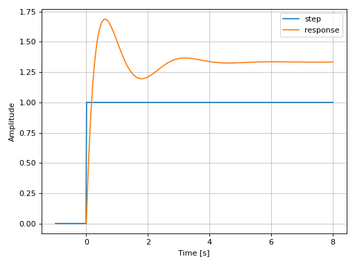

Plotting a MIMO system:

from sympy.physics.control.lti import TransferFunctionMatrix
tf1 = TransferFunction(1, s + 2, s)
tf2 = TransferFunction(s + 1, s**2 + s + 1, s)
tf3 = TransferFunction(s + 1, s**2 + s + 1.5, s)
tfm = TransferFunctionMatrix(
    [[tf1, -tf1], [tf2, -tf2], [tf3, -tf3]])
graphics(
    step_response(tfm),
    xlabel="Time [s]", ylabel="Amplitude"
)

(Source code, png)

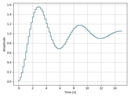
Plotting a discrete-time system:

import control as ct
G = ct.tf([0.0244, 0.0236], [1.1052, -2.0807, 1.0236], dt=0.2)
graphics(
    step_response(G, upper_limit=15),
    xlabel="Time [s]", ylabel="Amplitude"
)

(Source code, png)

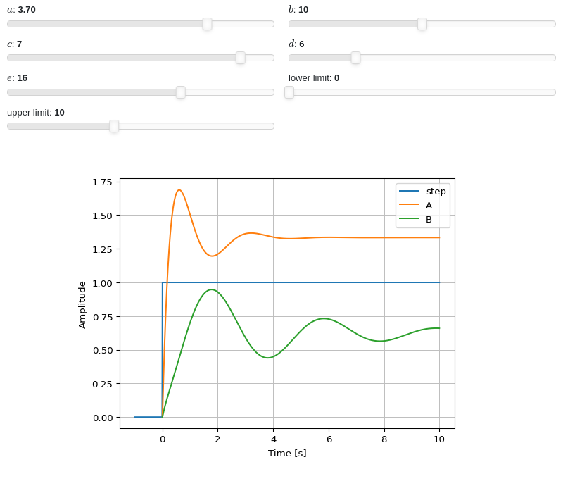
Interactive-widgets plot of multiple systems, one of which is parametric. A few observations:

The first system’s response will be computed with SymPy because control=False was set.
The second system’s response will be computed with the control module, because control=True was set.
Note the use of parametric lower_limit and upper_limit.
By moving the “lower limit” slider, the first system (evaluated with SymPy) will start from some amplitude value. However, on the second system (evaluated with the control module), the amplitude always starts from 0. That’s because the numerical integration’s initial condition is 0. Hence, if lower_limit is to be used, please set control=False.

from sympy.abc import a, b, c, d, e, f, g, s, t
from sympy import Heaviside
from sympy.physics.control.lti import TransferFunction
from spb import *
tf1 = TransferFunction(8*s**2 + 18*s + 32, s**3 + 6*s**2 + 14*s + 24, s)
tf2 = TransferFunction(s**2 + a*s + b, s**3 + c*s**2 + d*s + e, s)
params = {
    a: (3.7, 0, 5),
    b: (10, 0, 20),
    c: (7, 0, 8),
    d: (6, 0, 25),
    e: (16, 0, 25),
    f: (0, 0, 10, 50, "lower limit"),
    g: (10, 0, 25, 50, "upper limit"),
}
graphics(
    line(Heaviside(t), (t, -1, 10), label="step"),
    step_response(
        tf1, label="A", lower_limit=f, upper_limit=g, params=params,
        control=False),
    step_response(
        tf2, label="B", lower_limit=f, upper_limit=g, params=params,
        control=True),
    xlabel="Time [s]", ylabel="Amplitude"
)

(Source code, small.png)

spb.graphics.control.ramp_response(system, prec=8, slope=1, lower_limit=None, upper_limit=None, label=None, rendering_kw=None, control=True, input=None, output=None, **kwargs)[source]

Returns the ramp response of a continuous-time system.

Ramp function is defined as the straight line passing through origin (\(f(x) = mx\)). The slope of the ramp function can be varied by the user and the default value is 1.

Parameters:

systemLTI system type

The system for which the ramp response plot is to be computed. It can be:

an instance of sympy.physics.control.lti.TransferFunction or sympy.physics.control.lti.TransferFunctionMatrix
an instance of control.TransferFunction
an instance of scipy.signal.TransferFunction
a symbolic expression in rational form, which will be converted to an object of type sympy.physics.control.lti.TransferFunction.
a tuple of two or three elements: (num, den, generator [opt]), which will be converted to an object of type sympy.physics.control.lti.TransferFunction.

precint, optional

The decimal point precision for the point coordinate values. Defaults to 8.

slopeNumber, optional

The slope of the input ramp function. Defaults to 1.

lower_limitNumber or None, optional

The lower time limit of the plot range. Defaults to 0. If a different value is to be used, also set control=False (see examples in order to understand why).

upper_limitNumber or None, optional

The upper time limit of the plot range. If not provided, an appropriate value will be computed. If a interactive widget plot is being created, it defaults to 10.

labelstr, optional

The label to be shown on the legend.

rendering_kwdict, optional

A dictionary of keywords/values which is passed to the backend’s function to customize the appearance of lines. Refer to the plotting library (backend) manual for more informations.

controlbool, optional

If True, computes the ramp response with the control module, which uses numerical integration. If False, computes the ramp response with sympy, which uses the inverse Laplace transform. Default to True.

control_kwdict, optional

A dictionary of keyword arguments passed to control.forced_response()

inputint, optional

Only compute the ramp response for the listed input. If not specified, the ramp responses for each independent input are computed (as separate traces).

outputint, optional

Only compute the ramp response for the listed output. If not specified, all outputs are reported.

**kwargs

Keyword arguments are the same as line(). Refer to its documentation for a for a full list of keyword arguments.

Returns:

A list containing one or more instances of:

LineOver1DRangeSeries if control=False.
SystemResponseSeries if control=True.

See also

plot_step_response, plot_impulse_response

References

[1]

https://en.wikipedia.org/wiki/Ramp_function

Examples

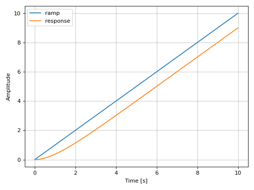
Plotting a SISO system:

from sympy.abc import s, t
from sympy.physics.control.lti import TransferFunction
from spb import *
tf1 = TransferFunction(1, (s+1), s)
ul = 10
graphics(
    line(t, (t, 0, ul), label="ramp"),
    ramp_response(tf1, upper_limit=ul, label="response"),
    xlabel="Time [s]", ylabel="Amplitude"
)

(Source code, png)

Plotting a MIMO system:

from sympy.physics.control.lti import TransferFunctionMatrix
tf1 = TransferFunction(1, s + 2, s)
tf2 = TransferFunction(s + 1, s**2 + s + 1, s)
tf3 = TransferFunction(s + 1, s**2 + s + 1.5, s)
tfm = TransferFunctionMatrix(
    [[tf1, -tf1], [tf2, -tf2], [tf3, -tf3]])
graphics(
    ramp_response(tfm),
    xlabel="Time [s]", ylabel="Amplitude"
)

(Source code, png)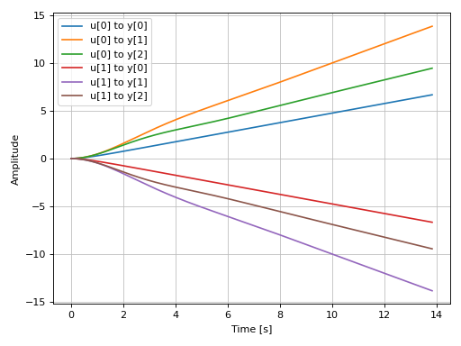

Plotting a discrete-time system:

import control as ct
G = ct.tf([0.0244, 0.0236], [1.1052, -2.0807, 1.0236], dt=0.2)
graphics(
    ramp_response(G, upper_limit=15),
    xlabel="Time [s]", ylabel="Amplitude"
)

(Source code, png)

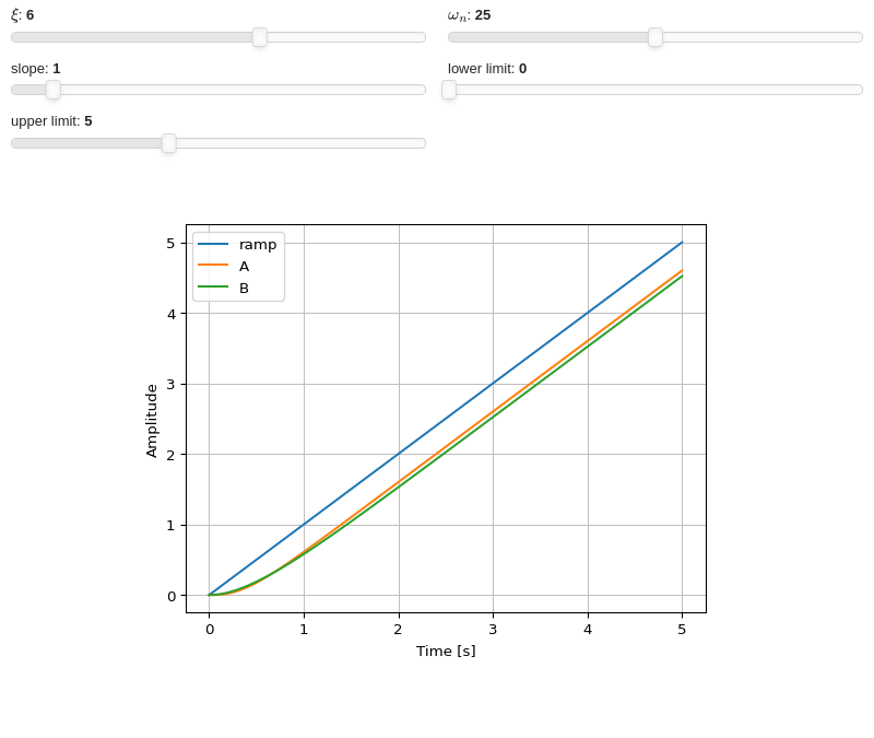
Interactive-widgets plot of multiple systems, one of which is parametric. A few observations:

The first system’s response will be computed with SymPy because control=False was set.
The second system’s response will be computed with the control module, because control=True was set.
Note the use of parametric lower_limit and upper_limit.
By moving the “lower limit” slider, the first system (evaluated with SymPy) will start from some amplitude value. However, on the second system (evaluated with the control module), the amplitude always starts from 0. That’s because the numerical integration’s initial condition is 0. Hence, if lower_limit is to be used, please set control=False.

from sympy import symbols
from sympy.physics.control.lti import TransferFunction
from spb import *
a, b, c, xi, wn, s, t = symbols("a, b, c, xi, omega_n, s, t")
tf1 = TransferFunction(25, s**2 + 10*s + 25, s)
tf2 = TransferFunction(wn**2, s**2 + 2*xi*wn*s + wn**2, s)
params = {
    xi: (6, 0, 10),
    wn: (25, 0, 50),
    a: (1, 0, 10, 50, "slope"),
    b: (0, 0, 5, 50, "lower limit"),
    c: (5, 2, 10, 50, "upper limit"),
}
graphics(
    line(a*t, (t, 0, c), params=params, label="ramp"),
    ramp_response(
        tf1, label="A", slope=a, lower_limit=b, upper_limit=c,
        params=params, control=False),
    ramp_response(
        tf2, label="B", slope=a, lower_limit=b, upper_limit=c,
        params=params, control=True),
    xlabel="Time [s]", ylabel="Amplitude")

(Source code, small.png)

spb.graphics.control.bode_magnitude(system, initial_exp=None, final_exp=None, freq_unit='rad/sec', phase_unit='rad', label=None, rendering_kw=None, input=None, output=None, **kwargs)[source]

Returns the Bode magnitude plot of a continuous-time system.

Parameters:

systemLTI system type

The system for which the step response plot is to be computed. It can be:

an instance of sympy.physics.control.lti.TransferFunction or sympy.physics.control.lti.TransferFunctionMatrix
an instance of control.TransferFunction
an instance of scipy.signal.TransferFunction
a symbolic expression in rational form, which will be converted to an object of type sympy.physics.control.lti.TransferFunction.
a tuple of two or three elements: (num, den, generator [opt]), which will be converted to an object of type sympy.physics.control.lti.TransferFunction.

initial_expNumber, optional

The initial exponent of 10 of the semilog plot. Default to None, which will autocompute the appropriate value.

final_expNumber, optional

The final exponent of 10 of the semilog plot. Default to None, which will autocompute the appropriate value.

precint, optional

The decimal point precision for the point coordinate values. Defaults to 8.

freq_unitstring, optional

User can choose between 'rad/sec' (radians/second) and 'Hz' (Hertz) as frequency units.

labelstr, optional

The label to be shown on the legend.

rendering_kwdict, optional

A dictionary of keywords/values which is passed to the backend’s function to customize the appearance of lines. Refer to the plotting library (backend) manual for more informations.

inputint, optional

Only compute the poles/zeros for the listed input. If not specified, the poles/zeros for each independent input are computed (as separate traces).

outputint, optional

Only compute the poles/zeros for the listed output. If not specified, all outputs are reported.

**kwargs

Keyword arguments are the same as line(). Refer to its documentation for a for a full list of keyword arguments.

Returns:

A list containing one instance of LineOver1DRangeSeries.

See also

bode_phase, nyquist, nichols, spb.plot_functions.control.plot_bode

Notes

plot_bode() returns a plotgrid() of two visualizations, one with the Bode magnitude, the other with the Bode phase.

Examples

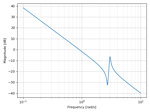
Bode magnitude plot of a continuous-time system:

from sympy.abc import s
from sympy.physics.control.lti import TransferFunction
from spb import *
tf1 = TransferFunction(
    1*s**2 + 0.1*s + 7.5, 1*s**4 + 0.12*s**3 + 9*s**2, s)
graphics(
    bode_magnitude(tf1),
    xscale="log", xlabel="Frequency [rad/s]",
    ylabel="Magnitude [dB]"
)

(Source code, png)

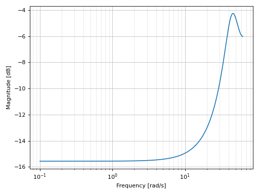
Bode magnitude plot of a discrete-time system:

import control as ct
tf2 = ct.tf([1], [1, 2, 3], dt=0.05)
graphics(
    bode_magnitude(tf2),
    xscale="log", xlabel="Frequency [rad/s]",
    ylabel="Magnitude [dB]"
)

(Source code, png)

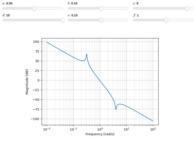
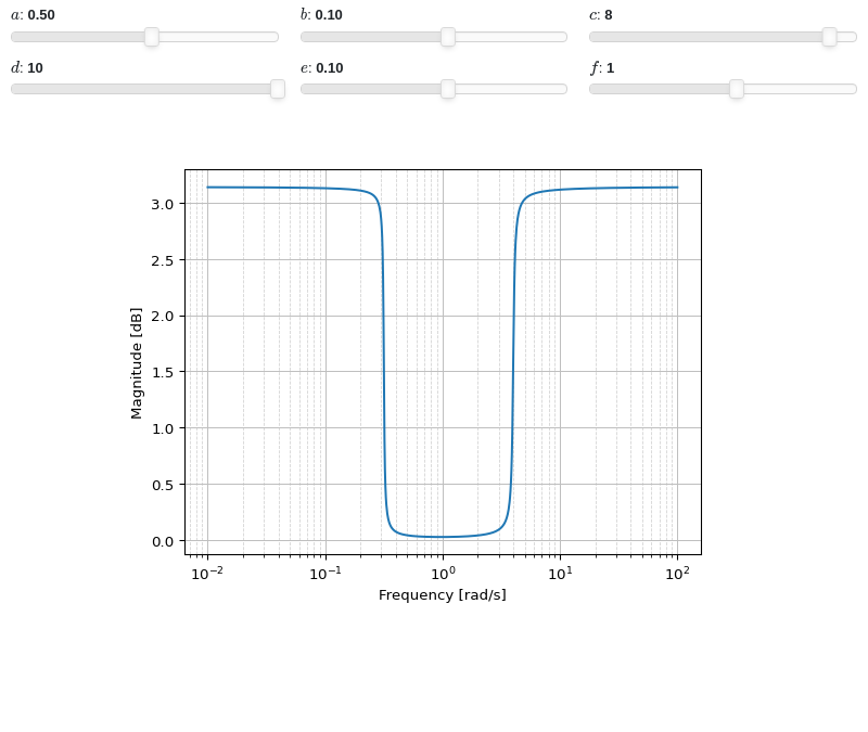
Interactive-widget plot:

from sympy.abc import a, b, c, d, e, f, s
from sympy.physics.control.lti import TransferFunction
from spb import *
tf1 = TransferFunction(a*s**2 + b*s + c, d*s**4 + e*s**3 + f*s**2, s)
params = {
    a: (0.5, -10, 10),
    b: (0.1, -1, 1),
    c: (8, -10, 10),
    d: (10, -10, 10),
    e: (0.1, -1, 1),
    f: (1, -10, 10),
}
graphics(
    bode_magnitude(tf1, initial_exp=-2, final_exp=2, params=params),
    imodule="panel", ncols=3,
    xscale="log", xlabel="Frequency [rad/s]", ylabel="Magnitude [dB]"
)

(Source code, small.png)

spb.graphics.control.bode_phase(system, initial_exp=None, final_exp=None, freq_unit='rad/sec', phase_unit='rad', label=None, rendering_kw=None, unwrap=True, input=None, output=None, **kwargs)[source]

Returns the Bode phase plot of a continuous-time system.

Parameters:

systemLTI system type

The system for which the step response plot is to be computed. It can be:

an instance of sympy.physics.control.lti.TransferFunction or sympy.physics.control.lti.TransferFunctionMatrix
an instance of control.TransferFunction
an instance of scipy.signal.TransferFunction
a symbolic expression in rational form, which will be converted to an object of type sympy.physics.control.lti.TransferFunction.
a tuple of two or three elements: (num, den, generator [opt]), which will be converted to an object of type sympy.physics.control.lti.TransferFunction.

initial_expNumber, optional

The initial exponent of 10 of the semilog plot. Default to None, which will autocompute the appropriate value.

final_expNumber, optional

The final exponent of 10 of the semilog plot. Default to None, which will autocompute the appropriate value.

precint, optional

The decimal point precision for the point coordinate values. Defaults to 8.

freq_unitstring, optional

User can choose between 'rad/sec' (radians/second) and 'Hz' (Hertz) as frequency units.

phase_unitstring, optional

User can choose between 'rad' (radians) and 'deg' (degree) as phase units.

unwrapbool, optional

Depending on the transfer function, the computed phase could contain discontinuities of 2*pi. unwrap=True post-process the numerical data in order to get a continuous phase. Default to True.

labelstr, optional

The label to be shown on the legend.

rendering_kwdict, optional

A dictionary of keywords/values which is passed to the backend’s function to customize the appearance of lines. Refer to the plotting library (backend) manual for more informations.

inputint, optional

Only compute the poles/zeros for the listed input. If not specified, the poles/zeros for each independent input are computed (as separate traces).

outputint, optional

Only compute the poles/zeros for the listed output. If not specified, all outputs are reported.

**kwargs

Keyword arguments are the same as line(). Refer to its documentation for a for a full list of keyword arguments.

Returns:

A list containing one instance of LineOver1DRangeSeries.

See also

bode_magnitude, nyquist, nichols

Notes

plot_bode() returns a plotgrid() of two visualizations, one with the Bode magnitude, the other with the Bode phase.

Examples

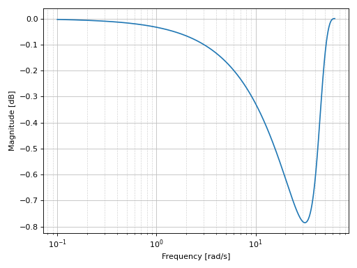
Bode phase plot of a continuous-time system:

from sympy.abc import s
from sympy.physics.control.lti import TransferFunction
from spb import *
tf1 = TransferFunction(
    1*s**2 + 0.1*s + 7.5, 1*s**4 + 0.12*s**3 + 9*s**2, s)
graphics(
    bode_phase(tf1, initial_exp=0.2, final_exp=0.7),
    xscale="log", xlabel="Frequency [rad/s]",
    ylabel="Magnitude [dB]"
)

(Source code, png)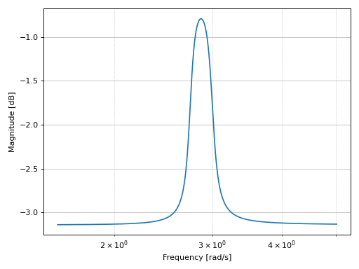

Bode phase plot of a discrete-time system:

import control as ct
tf2 = ct.tf([1], [1, 2, 3], dt=0.05)
graphics(
    bode_phase(tf2),
    xscale="log", xlabel="Frequency [rad/s]",
    ylabel="Magnitude [dB]"
)

(Source code, png)

Interactive-widget plot:

from sympy.abc import a, b, c, d, e, f, s
from sympy.physics.control.lti import TransferFunction
from spb import *
tf1 = TransferFunction(a*s**2 + b*s + c, d*s**4 + e*s**3 + f*s**2, s)
params = {
    a: (0.5, -10, 10),
    b: (0.1, -1, 1),
    c: (8, -10, 10),
    d: (10, -10, 10),
    e: (0.1, -1, 1),
    f: (1, -10, 10),
}
graphics(
    bode_phase(tf1, initial_exp=-2, final_exp=2, params=params),
    imodule="panel", ncols=3,
    xscale="log", xlabel="Frequency [rad/s]", ylabel="Magnitude [dB]"
)

(Source code, small.png)

spb.graphics.control.nyquist(system, omega_limits=None, input=None, output=None, label=None, rendering_kw=None, m_circles=False, **kwargs)[source]

Plots a Nyquist plot for the system over a (optional) frequency range. The curve is computed by evaluating the Nyquist segment along the positive imaginary axis, with a mirror image generated to reflect the negative imaginary axis. Poles on or near the imaginary axis are avoided using a small indentation. The portion of the Nyquist contour at infinity is not explicitly computed (since it maps to a constant value for any system with a proper transfer function).

Parameters:

systemLTI system type

The system for which the step response plot is to be computed. It can be:

an instance of sympy.physics.control.lti.TransferFunction or sympy.physics.control.lti.TransferFunctionMatrix
an instance of control.TransferFunction
an instance of scipy.signal.TransferFunction
a symbolic expression in rational form, which will be converted to an object of type sympy.physics.control.lti.TransferFunction.
a tuple of two or three elements: (num, den, generator [opt]), which will be converted to an object of type sympy.physics.control.lti.TransferFunction.

labelstr, optional

The label to be shown on the legend.

arrowsint or 1D/2D array of floats, optional

Specify the number of arrows to plot on the Nyquist curve. If an integer is passed, that number of equally spaced arrows will be plotted on each of the primary segment and the mirror image. If a 1D array is passed, it should consist of a sorted list of floats between 0 and 1, indicating the location along the curve to plot an arrow.

max_curve_magnitudefloat, optional

Restrict the maximum magnitude of the Nyquist plot to this value. Portions of the Nyquist plot whose magnitude is restricted are plotted using a different line style.

max_curve_offsetfloat, optional

When plotting scaled portion of the Nyquist plot, increase/decrease the magnitude by this fraction of the max_curve_magnitude to allow any overlaps between the primary and mirror curves to be avoided.

mirror_style[str, str] or [dict, dict] or dict or False, optional

Linestyles for mirror image of the Nyquist curve. If a list is given, the first element is used for unscaled portions of the Nyquist curve, the second element is used for portions that are scaled (using max_curve_magnitude). dict is a dictionary of keyword arguments to be passed to the plotting function, for example to plt.plot. If False then omit completely. Default linestyle is [’–’, ‘:’].

m_circlesbool or float or iterable, optional

Turn on/off M-circles, which are circles of constant closed loop magnitude. If float or iterable (of floats), represents specific magnitudes in dB.

primary_style[str, str] or [dict, dict] or dict, optional

Linestyles for primary image of the Nyquist curve. If a list is given, the first element is used for unscaled portions of the Nyquist curve, the second element is used for portions that are scaled (using max_curve_magnitude). dict is a dictionary of keyword arguments to be passed to the plotting function, for example to Matplotlib’s plt.plot. Default linestyle is [‘-’, ‘-.’].

omega_limitsarray_like of two values, optional

Limits to the range of frequencies.

start_markerstr or dict, optional

Marker to use to mark the starting point of the Nyquist plot. If dict is provided, it must containts keyword arguments to be passed to the plot function, for example to Matplotlib’s plt.plot.

control_kwdict, optional

A dictionary of keyword arguments passed to control.nyquist_response()

Returns:

A list containing:

one instance of MCirclesSeries if mcircles=True.
one instance of NyquistLineSeries.

See also

bode, nichols, mcircles

Notes

If a continuous-time system contains poles on or near the imaginary axis, a small indentation will be used to avoid the pole. The radius of the indentation is given by indent_radius and it is taken to the right of stable poles and the left of unstable poles. If a pole is exactly on the imaginary axis, the indent_direction parameter can be used to set the direction of indentation. Setting indent_direction to none will turn off indentation. If return_contour is True, the exact contour used for evaluation is returned.
For those portions of the Nyquist plot in which the contour is indented to avoid poles, resuling in a scaling of the Nyquist plot, the line styles are according to the settings of the primary_style and mirror_style keywords. By default the scaled portions of the primary curve use a dotted line style and the scaled portion of the mirror image use a dashdot line style.

References

[1]

https://en.wikipedia.org/wiki/Hall_circles

Examples

Plotting a single transfer function:

from sympy import Rational
from sympy.abc import s
from sympy.physics.control.lti import TransferFunction
from spb import *
tf1 = TransferFunction(
    4 * s**2 + 5 * s + 1, 3 * s**2 + 2 * s + 5, s)
graphics(
    nyquist(tf1, m_circles=True),
    xlabel="Real", ylabel="Imaginary",
    grid=False, aspect="equal"
)

(Source code, png)

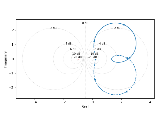
Visualizing M-circles:

graphics(
    nyquist(tf1, m_circles=True),
    grid=False, xlabel="Real", ylabel="Imaginary"
)

(Source code, png)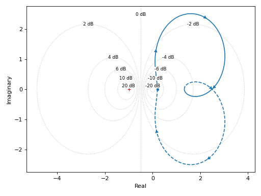

Interactive-widgets plot of a systems:

from sympy.abc import a, b, c, d, e, f, s
from sympy.physics.control.lti import TransferFunction
from spb import *
tf = TransferFunction(a * s**2 + b * s + c, d**2 * s**2 + e * s + f, s)
params = {
    a: (2, 0, 10),
    b: (5, 0, 10),
    c: (1, 0, 10),
    d: (1, 0, 10),
    e: (2, 0, 10),
    f: (3, 0, 10),
}
graphics(
    nyquist(tf, params=params),
    xlabel="Real", ylabel="Imaginary",
    xlim=(-1, 4), ylim=(-2.5, 2.5), aspect="equal"
)

(Source code, small.png)

spb.graphics.control.ngrid(cl_mags=None, cl_phases=None, label_cl_phases=False, rendering_kw=None, **kwargs)[source]

Create the n-grid (Nichols grid) of constant closed-loop magnitudes and phases.

Parameters:

cl_magsfloat or array-like (dB), optional: Array of closed-loop magnitudes defining the iso-gain lines. If False, hide closed-loop magnitude lines.
cl_phasesfloat or array-like (degrees), optional: Array of closed-loop phases defining the iso-phase lines. Must be in the range -360 < cl_phases < 0. If False, hide closed-loop phase lines.
label_cl_phases: bool, optional: If True, closed-loop phase lines will be labelled. Default to False.
rendering_kwdict or None, optional: A dictionary of keywords/values which is passed to the backend’s function to customize the appearance of lines. Refer to the plotting library (backend) manual for more informations.

Returns:

A list containing one instance of NGridLineSeries.

See also

nichols

Examples

Default N-grid:

from spb import *
graphics(
    ngrid(),
    grid=False
)

(Source code, png)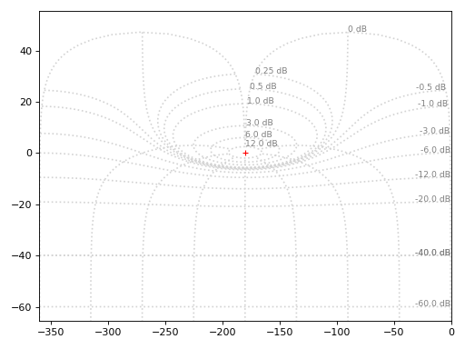

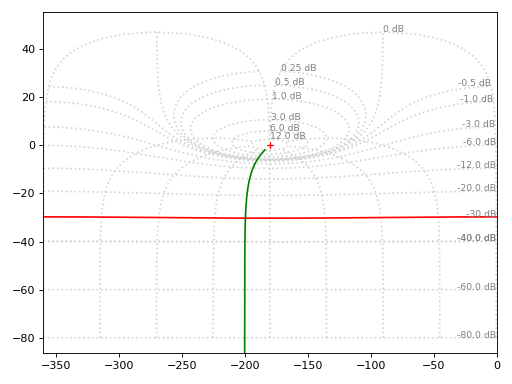
Highlight specific values of closed-loop magnitude and closed-loop phase:

graphics(
    ngrid(label_cl_phases=False),
    ngrid(cl_mags=-30, cl_phases=False, rendering_kw={"color": "r", "linestyle": "-"}),
    ngrid(cl_mags=False, cl_phases=-200, rendering_kw={"color": "g", "linestyle": "-"}),
    grid=False
)

(Source code, png)

spb.graphics.control.nichols(system, label=None, rendering_kw=None, ngrid=True, arrows=True, input=None, output=None, **kwargs)[source]

Nichols plot for a system over a (optional) frequency range.

Parameters:

systemLTI system type

The system for which the pole-zero plot is to be computed. It can be:

an instance of sympy.physics.control.lti.TransferFunction or sympy.physics.control.lti.TransferFunctionMatrix
an instance of control.TransferFunction
an instance of scipy.signal.TransferFunction
a symbolic expression in rational form, which will be converted to an object of type sympy.physics.control.lti.TransferFunction.
a tuple of two or three elements: (num, den, generator [opt]), which will be converted to an object of type sympy.physics.control.lti.TransferFunction.

arrowsbol, int or 1D array of floats, optional

Specify the number of arrows to plot on the Nichols curve. If an integer is passed, that number of equally spaced arrows will be plotted on each of the primary segment and the mirror image. If a 1D array is passed, it should consist of a sorted list of floats between 0 and 1, indicating the location along the curve to plot an arrow. If True, a default number of arrows is shown. If False, no arrows are shown.

ngridbool, optional

Turn on/off the [Nichols] grid lines.

omega_limitsarray_like of two values, optional

Limits to the range of frequencies.

labelstr, optional

The label to be shown on the legend.

rendering_kwdict, optional

A dictionary of keywords/values which is passed to the backend’s function to customize the appearance of lines. Refer to the plotting library (backend) manual for more informations.

inputint, optional

Only compute the poles/zeros for the listed input. If not specified, the poles/zeros for each independent input are computed (as separate traces).

outputint, optional

Only compute the poles/zeros for the listed output. If not specified, all outputs are reported.

**kwargs

Keyword arguments are the same as line_parametric_2d(). Refer to its documentation for a for a full list of keyword arguments.

Returns:

A list containing:

one instance of NGridLineSeries if ngrid=True.
one instance of NicholsLineSeries.

See also

bode_magnitude, bode_phase, nyquist, ngrid

References

[1]

https://en.wikipedia.org/wiki/Hall_circles

Examples

Plotting a single transfer function:

from sympy.abc import s
from sympy.physics.control.lti import TransferFunction
from spb import *
tf = TransferFunction(50*s**2 - 20*s + 15, -10*s**2 + 40*s + 30, s)
graphics(
    nichols(tf),
    xlabel="Open-Loop Phase [deg]",
    ylabel="Open-Loop Magnitude [dB]",
    grid=False
)

(Source code, png)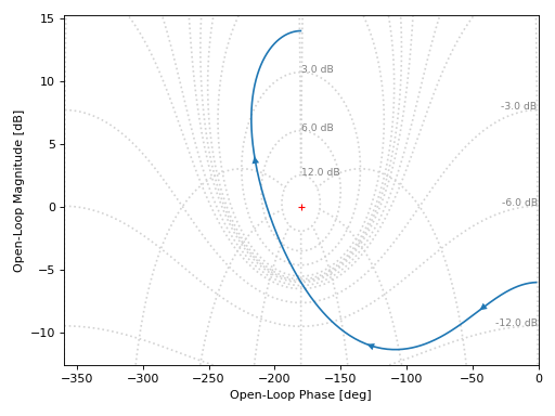

Turning off the Nichols grid lines:

graphics(
    nichols(tf, ngrid=False),
    xlabel="Open-Loop Phase [deg]",
    ylabel="Open-Loop Magnitude [dB]",
    grid=False
)

(Source code, png)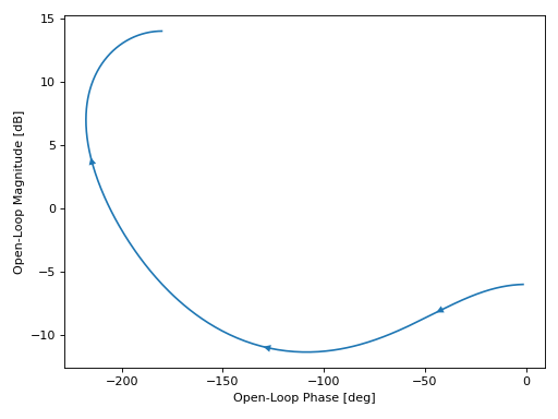

Interactive-widgets plot of a systems. For these kind of plots, it is recommended to set both omega_limits and xlim:

from sympy.abc import a, b, c, s
from spb import *
from sympy.physics.control.lti import TransferFunction
tf = TransferFunction(a*s**2 + b*s + c, s**3 + 10*s**2 + 5 * s + 1, s)
params = {
    a: (-25, -100, 100),
    b: (60, -300, 300),
    c: (-100, -1000, 1000),
}
graphics(
    nichols(tf, omega_limits=[1e-03, 1e03], n=1e04, params=params),
    xlabel="Open-Loop Phase [deg]",
    ylabel="Open-Loop Magnitude [dB]",
    xlim=(-360, 360), grid=False,
)

(Source code, small.png)

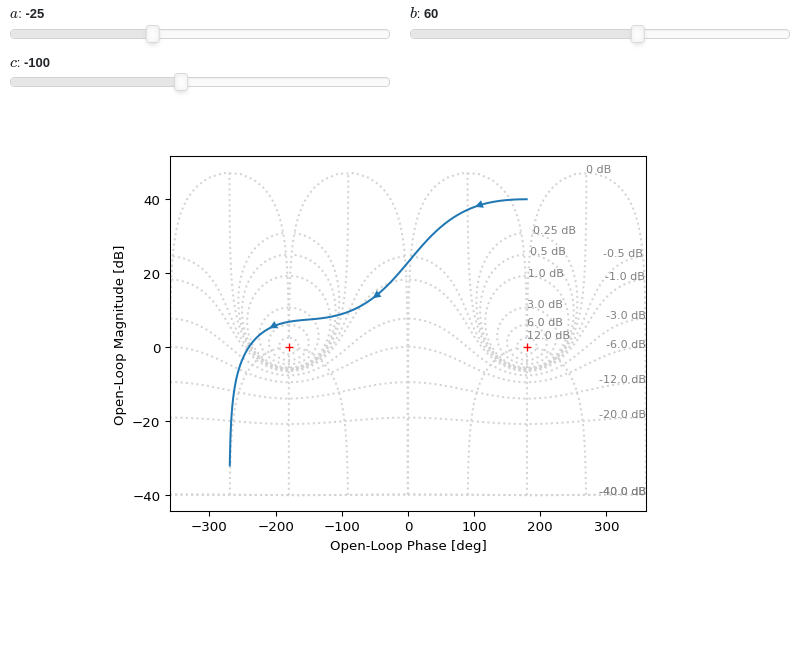
spb.graphics.control.mcircles(magnitudes_db=None, rendering_kw=None, show_minus_one=True, **kwargs)[source]

Draw M-circles of constant closed-loop magnitude.

Parameters:

magnitudes_dbfloat, iterable or None: Specify the magnitudes in dB. If None, a list of default magnitudes will be used.
rendering_kwdict or None, optional: A dictionary of keywords/values which is passed to the backend’s function to customize the appearance of lines. Refer to the plotting library (backend) manual for more informations.
show_minus_onebool: Show a marker at (x, y) = (-1, 0).

Returns:

A list containing one instance of MCirclesSeries.

See also

nyquist

Examples

from spb import *
graphics(
    mcircles(),
    mcircles(-3, rendering_kw={"color": "r"}),
    grid=False, aspect="equal")

(Source code, png)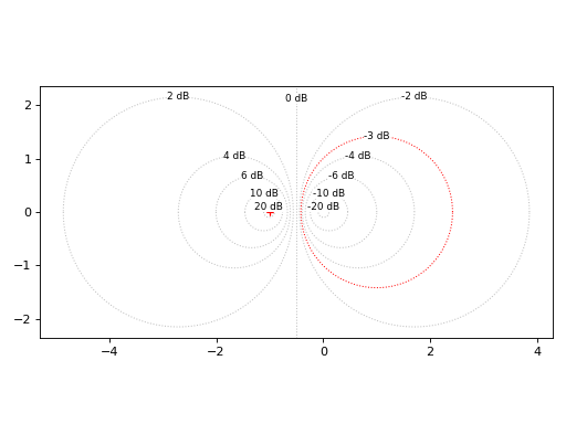

Interactive-widgets plot of m-circles:

from spb import *
from sympy.abc import m
graphics(
    mcircles(),
    mcircles(m, rendering_kw={"color": "r"}, params={m: (-3, -15, 15)}),
    grid=False, aspect="equal")

(Source code, small.png)

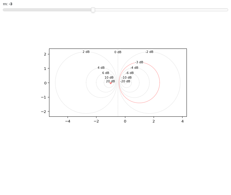
spb.graphics.control.control_axis(hor=True, ver=True, rendering_kw=None, **kwargs)[source]

Create two axis lines to be used with control-plotting.

Parameters:

hor, verbool, optional: Wheter to add the horizontal and/or vertical axis.
rendering_kwdict, optional: A dictionary of keywords/values which is passed to the backend’s function to customize the appearance of lines. Refer to the plotting library (backend) manual for more informations.

Returns:

A list containing up to two instances of HVLineSeries.

spb.graphics.control.sgrid(xi=None, wn=None, tp=None, ts=None, xlim=None, ylim=None, show_control_axis=True, rendering_kw=None, auto=False, **kwargs)[source]

Create the s-grid of constant damping ratios and natural frequencies.

Parameters:

xiiterable or float, optional: Damping ratios. Must be 0 <= xi <= 1. If None, default damping ratios will be used. If False, no damping ratios will be visualized.
wniterable or float, optional: Natural frequencies. If None, default natural frequencies will be used. If False, no natural frequencies will be visualized.
tpiterable or float, optional: Peak times.
tsiterable or float, optional: Settling times.
autobool, optional: If True, automatically compute damping ratio and natural frequencies in order to obtain a “evenly” distributed grid.
show_control_axisbool, optional: Shows an horizontal and vertical grid lines crossing at the origin. Default to True.
xlim, ylim2-elements tuple: If provided, compute damping ratios and natural frequencies in order to display “evenly” distributed grid lines on the plane.
rendering_kwdict, optional: A dictionary of keywords/values which is passed to the backend’s function to customize the appearance of lines. Refer to the plotting library (backend) manual for more informations.

See also

zgrid, pole_zero, root_locus

Examples

Shows the default grid lines, as well as a custom damping ratio line, a custom natural frequency line, a custom peak time line and a custom settling time line.

from spb import *
graphics(
    sgrid(),
    sgrid(xi=0.85, wn=False,
        rendering_kw={"color": "r", "linestyle": "-"},
        show_control_axis=False),
    sgrid(xi=False, wn=4.5,
        rendering_kw={"color": "g", "linestyle": "-"},
        show_control_axis=False),
    sgrid(xi=False, wn=False, tp=1,
        rendering_kw={"color": "b", "linestyle": "-"},
        show_control_axis=False),
    sgrid(xi=False, wn=False, ts=1,
        rendering_kw={"color": "m", "linestyle": "-"},
        show_control_axis=False),
    grid=False, xlim=(-8.5, 1), ylim=(-5, 5))

(Source code, png)

Auto-generate grid lines over a specified area of of the s-plane:

graphics(
    sgrid(auto=True)
)

(Source code, png)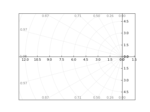

Interactive-widgets plot of custom s-grid lines:

from sympy import symbols
from spb import *
xi, wn, Tp, Ts = symbols("xi omega_n T_p T_s")
params = {
    xi: (0.85, 0, 1),
    wn: (6.5, 2, 8),
    Tp: (1, 0.2, 4),
    Ts: (1, 0.2, 4),
}
graphics(
    sgrid(auto=True),
    sgrid(xi=xi, wn=False, params=params,
        rendering_kw={"color": "r", "linestyle": "-"},
        show_control_axis=False),
    sgrid(xi=False, wn=wn, params=params,
        rendering_kw={"color": "g", "linestyle": "-"},
        show_control_axis=False),
    sgrid(xi=False, wn=False, tp=Tp, params=params,
        rendering_kw={"color": "b", "linestyle": "-"},
        show_control_axis=False),
    sgrid(xi=False, wn=False, ts=Ts, params=params,
        rendering_kw={"color": "m", "linestyle": "-"},
        show_control_axis=False),
    grid=False, xlim=(-8.5, 1), ylim=(-5, 5))

(Source code, small.png)

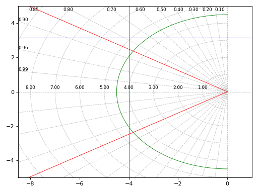
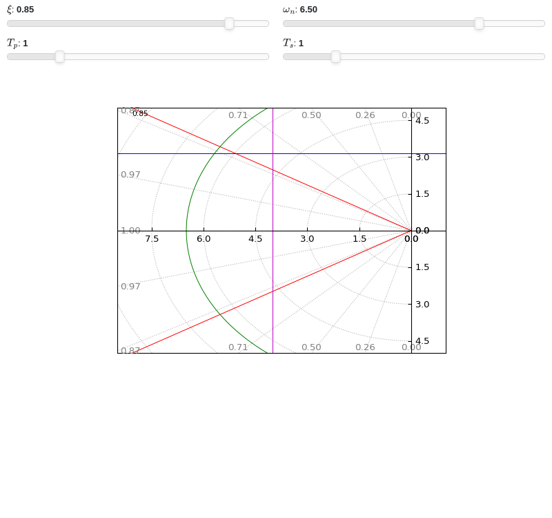
spb.graphics.control.zgrid(xi=None, wn=None, tp=None, ts=None, T=None, show_control_axis=True, rendering_kw=None, **kwargs)[source]

Create the s-grid of constant damping ratios and natural frequencies.

Parameters:

xiiterable or float, optional: Damping ratios. Must be 0 <= xi <= 1. If None, default damping ratios will be used. If False, no damping ratios will be visualized.
wniterable or float, optional: Normalized natural frequencies. If None, default natural frequencies will be used. If False, no natural frequencies will be visualized.
tpiterable or float, optional: Normalized peak times.
tsiterable or float, optional: Normalized settling times.
Tfloat or None, optional: Sampling period.
show_control_axisbool, optional: Shows an horizontal and vertical grid lines crossing at the origin. Default to True.
rendering_kwdict, optional: A dictionary of keywords/values which is passed to the backend’s function to customize the appearance of lines. Refer to the plotting library (backend) manual for more informations.

See also

sgrid, pole_zero, root_locus

Examples

Shows the default grid lines, as well as a custom damping ratio line and natural frequency line.

from spb import *
graphics(
    zgrid(),
    zgrid(xi=0.05, wn=False, rendering_kw={"color": "r", "linestyle": "-"}),
    zgrid(xi=False, wn=0.25, rendering_kw={"color": "b", "linestyle": "-"}),
    grid=False, aspect="equal", xlim=(-1.2, 1.2), ylim=(-1.2, 1.2))

(Source code, png)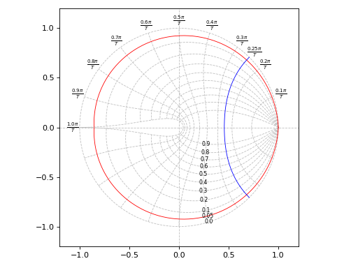

Shows a grid of settling times and peak times:

graphics(
    zgrid(xi=False, wn=False, tp=[3, 5, 7, 10, 20], ts=[2, 3, 5, 10, 20]),
    zgrid(xi=False, wn=False, tp=4, rendering_kw={"color": "r"}),
    zgrid(xi=False, wn=False, ts=7, rendering_kw={"color": "b"}),
    grid=False, aspect="equal", xlim=(-1.2, 1.2), ylim=(-1.2, 1.2))

(Source code, png)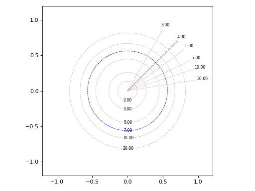

Interactive-widgets plot of z-grid lines:

from sympy import symbols
from spb import *
xi, wn, Tp, Ts = symbols("xi, omega_n, T_p, T_s")
graphics(
    zgrid(),
    zgrid(xi=xi, wn=False, rendering_kw={"color": "r", "linestyle": "-"}, params={xi: (0.05, 0, 1)}),
    zgrid(wn=wn, xi=False, rendering_kw={"color": "g", "linestyle": "-"}, params={wn: (0.45, 0, 1)}),
    zgrid(wn=False, xi=False, tp=Tp, rendering_kw={"color": "b", "linestyle": "-"}, params={Tp: (3, 0, 20)}),
    zgrid(wn=False, xi=False, ts=Ts, rendering_kw={"color": "m", "linestyle": "-"}, params={Ts: (5, 0, 20)}),
    grid=False, aspect="equal", xlabel="Real", ylabel="Imaginary")

(Source code, small.png)

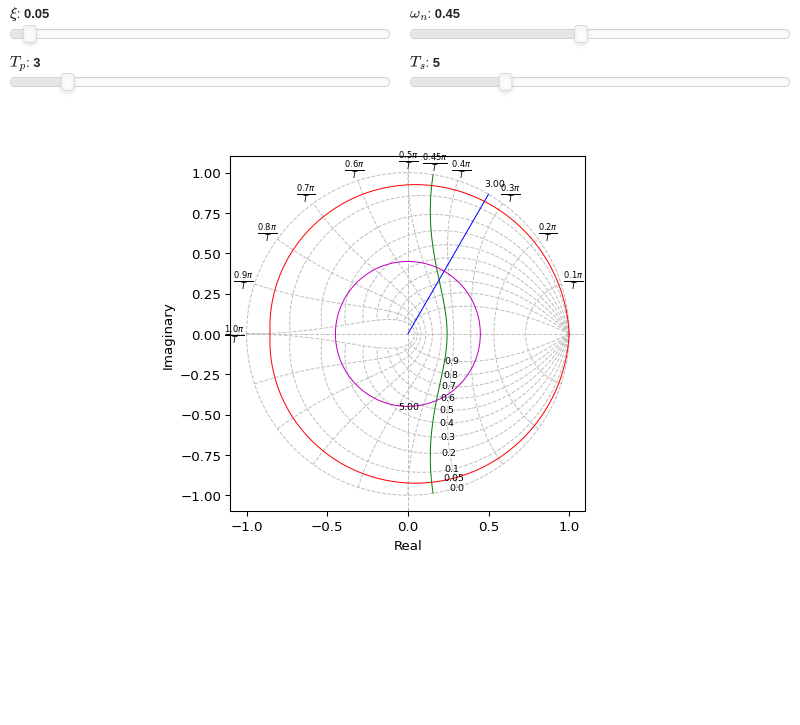
spb.graphics.control.root_locus(system, label=None, rendering_kw=None, rl_kw={}, sgrid=True, zgrid=False, input=None, output=None, **kwargs)[source]

Root Locus plot for a system.

Parameters:

systemLTI system type

The system for which the pole-zero plot is to be computed. It can be:

an instance of sympy.physics.control.lti.TransferFunction or sympy.physics.control.lti.TransferFunctionMatrix
an instance of control.TransferFunction
an instance of scipy.signal.TransferFunction
a symbolic expression in rational form, which will be converted to an object of type sympy.physics.control.lti.TransferFunction.
a tuple of two or three elements: (num, den, generator [opt]), which will be converted to an object of type sympy.physics.control.lti.TransferFunction.

labelstr, optional

The label to be shown on the legend.

rendering_kwdict, optional

A dictionary of keywords/values which is passed to the backend’s function to customize the appearance of lines. Refer to the plotting library (backend) manual for more informations.

control_kwdict

A dictionary of keyword arguments to be passed to control.root_locus_map().

sgridbool, optional

Generates a grid of constant damping ratios and natural frequencies on the s-plane. Default to True.

zgridbool, optional

Generates a grid of constant damping ratios and natural frequencies on the z-plane. Default to False. If zgrid=True, then it will automatically sets sgrid=False.

inputint, optional

Only compute the poles/zeros for the listed input. If not specified, the poles/zeros for each independent input are computed (as separate traces).

outputint, optional

Only compute the poles/zeros for the listed output. If not specified, all outputs are reported.

**kwargs

Keyword arguments are the same as line(). Refer to its documentation for a for a full list of keyword arguments.

Returns:

A list containing:

one instance of SGridLineSeries if sgrid=True.
one instance of ZGridLineSeries if zgrid=True.
one or more instances of RootLocusSeries.

See also

sgrid, zgrid, pole_zero

Examples

Plot the root locus of a system on the s-plane, also showing a custom damping ratio line.

from sympy.abc import s, z
from spb import *
G = (s**2 - 4) / (s**3 + 2*s - 3)
graphics(
    root_locus(G),
    sgrid(xi=0.92, wn=False, rendering_kw={"color": "r"}),
    grid=False, xlabel="Real", ylabel="Imaginary")

(Source code, png)

Plot the root locus of a discrete system on the z-plane:

G = (0.038*z + 0.031) / (9.11*z**2 - 13.77*z + 5.0)
graphics(
    root_locus(G, sgrid=False, aspect="equal"),
    zgrid(T=0.2),
    grid=False, xlabel="Real", ylabel="Imaginary")

(Source code, png)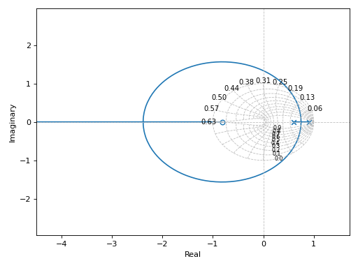

Interactive-widgets root locus plot:

from sympy import symbols
from spb import *
a, s, xi = symbols("a, s, xi")
G = (s**2 + a) / (s**3 + 2*s**2 + 3*s + 4)
params={a: (-0.5, -4, 4), xi: (0.8, 0, 1)}
graphics(
    sgrid(xi, wn=False, params=params, rendering_kw={"color": "r"}),
    root_locus(G, params=params),
    grid=False, xlim=(-4, 1), ylim=(-2.5, 2.5),
    xlabel="Real", ylabel="Imaginary")

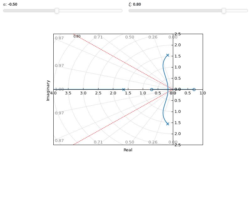
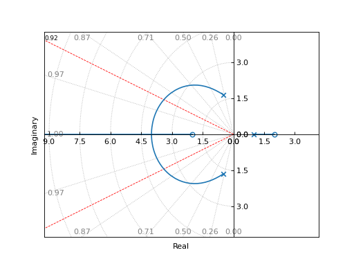(Source code, small.png)