Control
This module contains plotting functions for some of the common plots used in control system. In particular, the following functions:
make use of the functions defined in
spb.graphics.control.set axis labels to sensible choices.
Refer to Control for a general explanation about the underlying working principles, or if you are interested in a finer customization of what is shown on the plot.
NOTEs:
All the following examples are generated using Matplotlib. However, Bokeh can be used too, which allows for a better data exploration thanks to useful tooltips. Set
backend=BBin the function call to use Bokeh.For technical reasons, all interactive-widgets plots in this documentation are created using Holoviz’s Panel. Often, they will ran just fine with ipywidgets too. However, if a specific example uses the
paramlibrary, or widgets from thepanelmodule, then users will have to modify theparamsdictionary in order to make it work with ipywidgets. Refer to Interactive module for more information.
- spb.plot_functions.control.plot_pole_zero(*systems, pole_markersize=10, zero_markersize=7, show_axes=False, sgrid=False, zgrid=False, control=True, input=None, output=None, **kwargs)[source]
Returns the [Pole-Zero] plot (also known as PZ Plot or PZ Map) of a system.
A Pole-Zero plot is a graphical representation of a system’s poles and zeros. It is plotted on a complex plane, with circular markers representing the system’s zeros and ‘x’ shaped markers representing the system’s poles.
- Parameters:
- systemsone or more LTI system type
The system for which the pole-zero plot is to be computed. It can be:
an instance of
sympy.physics.control.lti.TransferFunctionorsympy.physics.control.lti.TransferFunctionMatrixan instance of
control.TransferFunctionan instance of
scipy.signal.TransferFunctiona symbolic expression in rational form, which will be converted to an object of type
sympy.physics.control.lti.TransferFunction.a tuple of two or three elements:
(num, den, generator [opt]), which will be converted to an object of typesympy.physics.control.lti.TransferFunction.a sequence of LTI systems.
a sequence of 2-tuples
(LTI system, label).a dict mapping LTI systems to labels.
- pole_colorstr, tuple, optional
The color of the pole points on the plot.
- pole_markersizeNumber, optional
The size of the markers used to mark the poles in the plot. Default pole markersize is 10.
- zero_colorstr, tuple, optional
The color of the zero points on the plot.
- zero_markersizeNumber, optional
The size of the markers used to mark the zeros in the plot. Default zero markersize is 7.
- z_rendering_kwdict
A dictionary of keyword arguments to further customize the appearance of zeros.
- p_rendering_kwdict
A dictionary of keyword arguments to further customize the appearance of poles.
- sgridbool, optional
Generates a grid of constant damping ratios and natural frequencies on the s-plane. Default to False.
- zgridbool, optional
Generates a grid of constant damping ratios and natural frequencies on the z-plane. Default to False.
- controlbool, optional
If True, computes the poles/zeros with the
controlmodule, which uses numerical integration. If False, computes them withsympy. Default to True.- inputint, optional
Only compute the poles/zeros for the listed input. If not specified, the poles/zeros for each independent input are computed (as separate traces).
- outputint, optional
Only compute the poles/zeros for the listed output. If not specified, all outputs are reported.
- **kwargsdict
Refer to
graphics()for a full list of keyword arguments to customize the appearances of the figure (title, axis labels, …).
References
Examples
Plotting poles and zeros on the s-plane:
from sympy.abc import s
from sympy import I
from sympy.physics.control.lti import TransferFunction
from spb import plot_pole_zero
tf1 = TransferFunction(
    s**2 + 1, s**4 + 4*s**3 + 6*s**2 + 5*s + 2, s)
plot_pole_zero(tf1, sgrid=True)
(
Source code,png)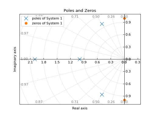
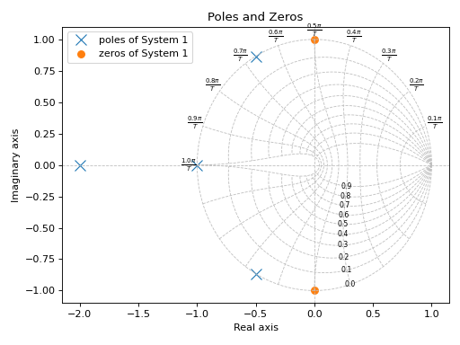
Plotting poles and zeros on the z-plane:
plot_pole_zero(tf1, zgrid=True)
(
Source code,png)
If a transfer function has complex coefficients, make sure to request the evaluation using
sympyinstead of thecontrolmodule:tf = TransferFunction(s + 2, s**2 + (2+I)*s + 10, s) plot_pole_zero(tf, control=False, grid=False, show_axes=True)
(
Source code,png)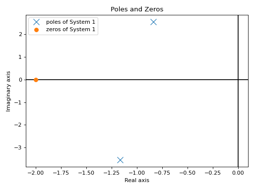
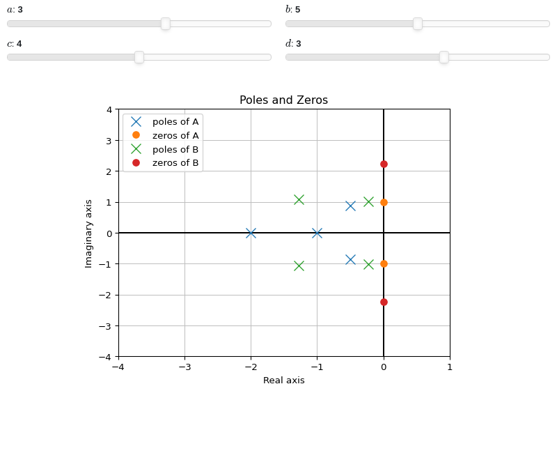
Interactive-widgets plot of multiple systems, one of which is parametric:
from sympy.abc import a, b, c, d, s
from sympy.physics.control.lti import TransferFunction
from spb import plot_pole_zero
tf1 = TransferFunction(s**2 + 1, s**4 + 4*s**3 + 6*s**2 + 5*s + 2, s)
tf2 = TransferFunction(s**2 + b, s**4 + a*s**3 + b*s**2 + c*s + d, s)
plot_pole_zero(
    (tf1, "A"), (tf2, "B"),
    params={
        a: (3, 0, 5),
        b: (5, 0, 10),
        c: (4, 0, 8),
        d: (3, 0, 5),
    },
    xlim=(-4, 1), ylim=(-4, 4),
    show_axes=True)

- spb.plot_functions.control.plot_step_response(*systems, lower_limit=None, upper_limit=None, prec=8, show_axes=False, control=True, input=None, output=None, **kwargs)[source]
Returns the unit step response of a continuous-time system. It is the response of the system when the input signal is a step function.
- Parameters:
- systemsLTI system type
The LTI system for which the step response is to be computed. It can be:
an instance of
sympy.physics.control.lti.TransferFunctionorsympy.physics.control.lti.TransferFunctionMatrixan instance of
control.TransferFunctionan instance of
scipy.signal.TransferFunctiona symbolic expression in rational form, which will be converted to an object of type
sympy.physics.control.lti.TransferFunction.a tuple of two or three elements:
(num, den, generator [opt]), which will be converted to an object of typesympy.physics.control.lti.TransferFunction.a sequence of LTI systems.
a sequence of 2-tuples
(LTI system, label).a dict mapping LTI systems to labels.
- lower_limitNumber or None, optional
The lower time limit of the plot range. Defaults to 0. If a different value is to be used, also set
control=False(see examples in order to understand why).- upper_limitNumber or None, optional
The upper time limit of the plot range. If not provided, an appropriate value will be computed. If a interactive widget plot is being created, it defaults to 10.
- precint, optional
The decimal point precision for the point coordinate values. Defaults to 8.
- show_axesboolean, optional
If
True, the coordinate axes will be shown. Defaults to False.- controlbool
If True, computes the step response with the
controlmodule, which uses numerical integration. If False, computes the step response withsympy, which uses the inverse Laplace transform. Default to True.- control_kwdict
A dictionary of keyword arguments passed to
control.step_response().- inputint, optional
Only compute the step response for the listed input. If not specified, the step responses for each independent input are computed (as separate traces).
- outputint, optional
Only compute the step response for the listed output. If not specified, all outputs are reported.
- **kwargsdict
Refer to
step_response()for a full list of keyword arguments to customize the appearances of lines.Refer to
graphics()for a full list of keyword arguments to customize the appearances of the figure (title, axis labels, …).
See also
References
Examples
Plotting a SISO system:
from sympy.abc import s
from sympy.physics.control.lti import TransferFunction
from spb import plot_step_response
tf1 = TransferFunction(8*s**2 + 18*s + 32, s**3 + 6*s**2 + 14*s + 24, s)
plot_step_response(tf1)
(
Source code,png)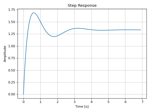
Plotting a MIMO system:
from sympy.physics.control.lti import TransferFunctionMatrix
tf1 = TransferFunction(1, s + 2, s)
tf2 = TransferFunction(s + 1, s**2 + s + 1, s)
tf3 = TransferFunction(s + 1, s**2 + s + 1.5, s)
tfm = TransferFunctionMatrix(
    [[tf1, -tf1], [tf2, -tf2], [tf3, -tf3]])
plot_step_response(tfm)
(
Source code,png)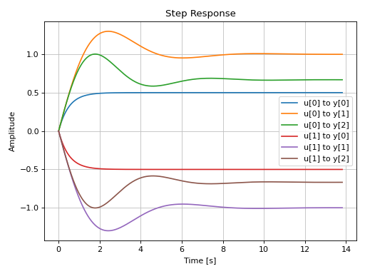
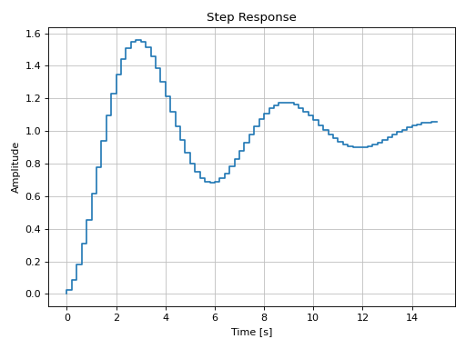
Plotting a discrete-time system:
import control as ct
G = ct.tf([0.0244, 0.0236], [1.1052, -2.0807, 1.0236], dt=0.2)
plot_step_response(G, upper_limit=15)
(
Source code,png)
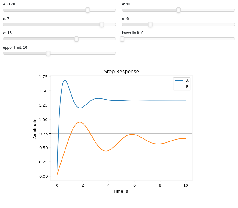
Interactive-widgets plot of multiple systems, one of which is parametric. A few observations:
Both systems are evaluated with the
controlmodule.Note the use of parametric
lower_limitandupper_limit.By moving the “lower limit” slider, both systems always start from zero amplitude. That’s because the numerical integration’s initial condition is 0. Hence, if
lower_limitis to be used, please setcontrol=False.
from sympy.abc import a, b, c, d, e, f, g, s
from sympy.physics.control.lti import TransferFunction
from spb import plot_step_response
tf1 = TransferFunction(8*s**2 + 18*s + 32, s**3 + 6*s**2 + 14*s + 24, s)
tf2 = TransferFunction(s**2 + a*s + b, s**3 + c*s**2 + d*s + e, s)
plot_step_response(
    (tf1, "A"), (tf2, "B"), lower_limit=f, upper_limit=g,
    params={
        a: (3.7, 0, 5),
        b: (10, 0, 20),
        c: (7, 0, 8),
        d: (6, 0, 25),
        e: (16, 0, 25),
        f: (0, 0, 10, 50, "lower limit"),
        g: (10, 0, 25, 50, "upper limit"),
    })

- spb.plot_functions.control.plot_impulse_response(*systems, prec=8, lower_limit=None, upper_limit=None, show_axes=False, control=True, input=None, output=None, **kwargs)[source]
Returns the unit impulse response (Input is the Dirac-Delta Function) of a continuous-time system.
- Parameters:
- systemsLTI system type
The LTI system for which the impulse response is to be computed. It can be:
an instance of
sympy.physics.control.lti.TransferFunctionorsympy.physics.control.lti.TransferFunctionMatrixan instance of
control.TransferFunctionan instance of
scipy.signal.TransferFunctiona symbolic expression in rational form, which will be converted to an object of type
sympy.physics.control.lti.TransferFunction.a tuple of two or three elements:
(num, den, generator [opt]), which will be converted to an object of typesympy.physics.control.lti.TransferFunction.a sequence of LTI systems.
a sequence of 2-tuples
(LTI system, label).a dict mapping LTI systems to labels.
- lower_limitNumber or None, optional
The lower time limit of the plot range. Defaults to 0. If a different value is to be used, also set
control=False(see examples in order to understand why).- upper_limitNumber or None, optional
The upper time limit of the plot range. If not provided, an appropriate value will be computed. If a interactive widget plot is being created, it defaults to 10.
- precint, optional
The decimal point precision for the point coordinate values. Defaults to 8.
- show_axesboolean, optional
If
True, the coordinate axes will be shown. Defaults to False.- controlbool
If True, computes the step response with the
controlmodule, which uses numerical integration. If False, computes the step response withsympy, which uses the inverse Laplace transform. Default to True.- control_kwdict
A dictionary of keyword arguments passed to
control.impulse_response().- inputint, optional
Only compute the impulse response for the listed input. If not specified, the impulse responses for each independent input are computed (as separate traces).
- outputint, optional
Only compute the impulse response for the listed output. If not specified, all outputs are reported.
- **kwargsdict
Refer to
impulse_response()for a full list of keyword arguments to customize the appearances of lines.Refer to
graphics()for a full list of keyword arguments to customize the appearances of the figure (title, axis labels, …).
See also
References
Examples
Plotting a SISO system:
from sympy.abc import s
from sympy.physics.control.lti import TransferFunction
from spb import plot_impulse_response
tf1 = TransferFunction(
    8*s**2 + 18*s + 32, s**3 + 6*s**2 + 14*s + 24, s)
plot_impulse_response(tf1)
(
Source code,png)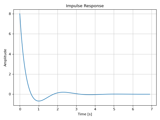
Plotting a MIMO system:
from sympy.physics.control.lti import TransferFunctionMatrix
tf1 = TransferFunction(1, s + 2, s)
tf2 = TransferFunction(s + 1, s**2 + s + 1, s)
tf3 = TransferFunction(s + 1, s**2 + s + 1.5, s)
tfm = TransferFunctionMatrix(
    [[tf1, -tf1], [tf2, -tf2], [tf3, -tf3]])
plot_impulse_response(tfm)
(
Source code,png)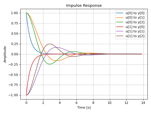
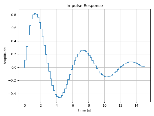
Plotting a discrete-time system:
import control as ct
G = ct.tf([0.0244, 0.0236], [1.1052, -2.0807, 1.0236], dt=0.2)
plot_impulse_response(G, upper_limit=15)
(
Source code,png)
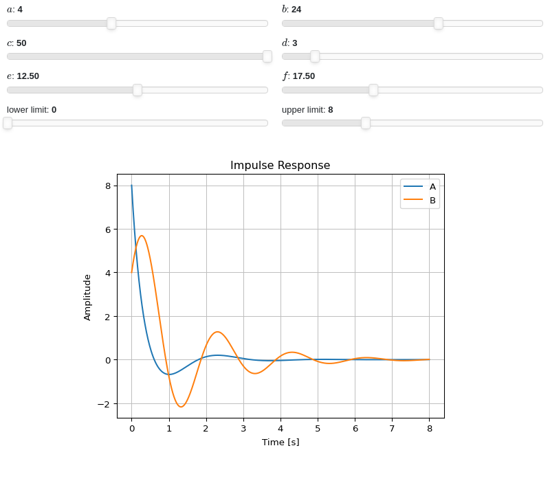
Interactive-widgets plot of multiple systems, one of which is parametric. A few observations:
Both systems are evaluated with the
controlmodule.Note the use of parametric
lower_limitandupper_limit.By moving the “lower limit” slider, both systems always start from zero amplitude. That’s because the numerical integration’s initial condition is 0. Hence, if
lower_limitis to be used, please setcontrol=False.
from sympy.abc import a, b, c, d, e, f, g, h, s
from sympy.physics.control.lti import TransferFunction
from spb import plot_impulse_response
tf1 = TransferFunction(8*s**2 + 18*s + 32, s**3 + 6*s**2 + 14*s + 24, s)
tf2 = TransferFunction(a*s**2 + b*s + c, s**3 + d*s**2 + e*s + f, s)
plot_impulse_response(
    (tf1, "A"), (tf2, "B"), lower_limit=g, upper_limit=h,
    params={
        a: (4, 0, 10),
        b: (24, 0, 40),
        c: (50, 0, 50),
        d: (3, 0, 25),
        e: (12.5, 0, 25),
        f: (17.5, 0, 50),
        g: (0, 0, 10, 50, "lower limit"),
        h: (8, 0, 25, 50, "upper limit"),
    })

- spb.plot_functions.control.plot_ramp_response(*systems, slope=1, prec=8, lower_limit=None, upper_limit=None, show_axes=False, control=True, input=None, output=None, **kwargs)[source]
Returns the ramp response of a continuous-time system.
Ramp function is defined as the straight line passing through origin (\(f(x) = mx\)). The slope of the ramp function can be varied by the user and the default value is 1.
- Parameters:
- systemsLTI system type
The LTI system for which the ramp response is to be computed. It can be:
an instance of
sympy.physics.control.lti.TransferFunctionorsympy.physics.control.lti.TransferFunctionMatrixan instance of
control.TransferFunctionan instance of
scipy.signal.TransferFunctiona symbolic expression in rational form, which will be converted to an object of type
sympy.physics.control.lti.TransferFunction.a tuple of two or three elements:
(num, den, generator [opt]), which will be converted to an object of typesympy.physics.control.lti.TransferFunction.a sequence of LTI systems.
a sequence of 2-tuples
(LTI system, label).a dict mapping LTI systems to labels.
- slopeNumber, optional
The slope of the input ramp function. Defaults to 1.
- lower_limitNumber or None, optional
The lower time limit of the plot range. Defaults to 0. If a different value is to be used, also set
control=False(see examples in order to understand why).- upper_limitNumber or None, optional
The upper time limit of the plot range. If not provided, an appropriate value will be computed. If a interactive widget plot is being created, it defaults to 10.
- precint, optional
The decimal point precision for the point coordinate values. Defaults to 8.
- show_axesboolean, optional
If
True, the coordinate axes will be shown. Defaults to False.- controlbool
If True, computes the step response with the
controlmodule, which uses numerical integration. If False, computes the step response withsympy, which uses the inverse Laplace transform. Default to True.- control_kwdict
A dictionary of keyword arguments passed to
control.forced_response().- inputint, optional
Only compute the ramp response for the listed input. If not specified, the ramp responses for each independent input are computed (as separate traces).
- outputint, optional
Only compute the ramp response for the listed output. If not specified, all outputs are reported.
- **kwargsdict
Refer to
ramp_response()for a full list of keyword arguments to customize the appearances of lines.Refer to
graphics()for a full list of keyword arguments to customize the appearances of the figure (title, axis labels, …).
See also
References
Examples
Plotting a SISO system:
from sympy.abc import s
from sympy.physics.control.lti import TransferFunction
from spb import plot_ramp_response
tf1 = TransferFunction(1, (s+1), s)
plot_ramp_response(tf1)
(
Source code,png)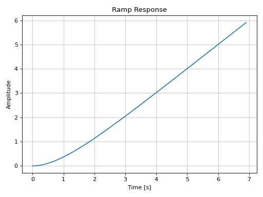
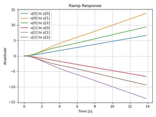
Plotting a MIMO system:
from sympy.physics.control.lti import TransferFunctionMatrix
tf1 = TransferFunction(1, s + 2, s)
tf2 = TransferFunction(s + 1, s**2 + s + 1, s)
tf3 = TransferFunction(s + 1, s**2 + s + 1.5, s)
tfm = TransferFunctionMatrix(
    [[tf1, -tf1], [tf2, -tf2], [tf3, -tf3]])
plot_ramp_response(tfm)
(
Source code,png)
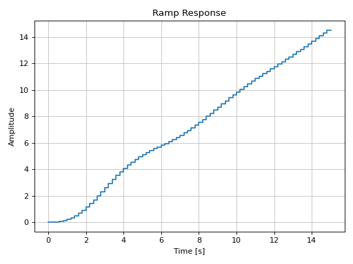
Plotting a discrete-time system:
import control as ct
G = ct.tf([0.0244, 0.0236], [1.1052, -2.0807, 1.0236], dt=0.2)
plot_ramp_response(G, upper_limit=15)
(
Source code,png)
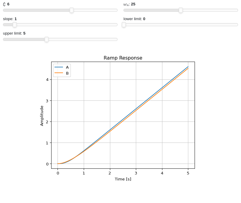
Interactive-widgets plot of multiple systems, one of which is parametric. A few observations:
Both systems are evaluated with the
controlmodule.Note the use of parametric
lower_limitandupper_limit.By moving the “lower limit” slider, both systems always start from zero amplitude. That’s because the numerical integration’s initial condition is 0. Hence, if
lower_limitis to be used, please setcontrol=False.
from sympy import symbols
from sympy.physics.control.lti import TransferFunction
from spb import plot_ramp_response
a, b, c, xi, wn, s, t = symbols("a, b, c, xi, omega_n, s, t")
tf1 = TransferFunction(25, s**2 + 10*s + 25, s)
tf2 = TransferFunction(wn**2, s**2 + 2*xi*wn*s + wn**2, s)
params = {
    xi: (6, 0, 10),
    wn: (25, 0, 50),
    a: (1, 0, 10, 50, "slope"),
    b: (0, 0, 5, 50, "lower limit"),
    c: (5, 2, 10, 50, "upper limit"),
}
plot_ramp_response(
    (tf1, "A"), (tf2, "B"),
    slope=a, lower_limit=b, upper_limit=c,
    params=params)

- spb.plot_functions.control.plot_bode_magnitude(*systems, initial_exp=None, final_exp=None, freq_unit=None, show_axes=False, **kwargs)[source]
Returns the Bode magnitude plot of a continuous-time system.
See
plot_bodefor all the parameters.
- spb.plot_functions.control.plot_bode_phase(*systems, initial_exp=None, final_exp=None, freq_unit=None, phase_unit=None, show_axes=False, unwrap=True, **kwargs)[source]
Returns the Bode phase plot of a continuous-time system.
See
plot_bodefor all the parameters.
- spb.plot_functions.control.plot_bode(*systems, initial_exp=None, final_exp=None, freq_unit=None, phase_unit=None, show_axes=False, unwrap=True, **kwargs)[source]
Returns the Bode phase and magnitude plots of a continuous-time system.
- Parameters:
- systemsLTI system type
The LTI system for which the ramp response is to be computed. It can be:
an instance of
sympy.physics.control.lti.TransferFunctionorsympy.physics.control.lti.TransferFunctionMatrixan instance of
control.TransferFunctionan instance of
scipy.signal.TransferFunctiona symbolic expression in rational form, which will be converted to an object of type
sympy.physics.control.lti.TransferFunction.a tuple of two or three elements:
(num, den, generator [opt]), which will be converted to an object of typesympy.physics.control.lti.TransferFunction.a sequence of LTI systems.
a sequence of 2-tuples
(LTI system, label).a dict mapping LTI systems to labels.
- initial_expNumber, optional
The initial exponent of 10 of the semilog plot. Default to None, which will autocompute the appropriate value.
- final_expNumber, optional
The final exponent of 10 of the semilog plot. Default to None, which will autocompute the appropriate value.
- precint, optional
The decimal point precision for the point coordinate values. Defaults to 8.
- show_axesboolean, optional
If
True, the coordinate axes will be shown. Defaults to False.- freq_unitstring, optional
User can choose between
'rad/sec'(radians/second) and'Hz'(Hertz) as frequency units.- phase_unitstring, optional
User can choose between
'rad'(radians) and'deg'(degree) as phase units.- unwrapbool, optional
Depending on the transfer function, the computed phase could contain discontinuities of 2*pi.
unwrap=Truepost-process the numerical data in order to get a continuous phase.- inputint, optional
Only compute the poles/zeros for the listed input. If not specified, the poles/zeros for each independent input are computed (as separate traces).
- outputint, optional
Only compute the poles/zeros for the listed output. If not specified, all outputs are reported. Default to True.
- **kwargsdict
Refer to
bode_magnitude()for a full list of keyword arguments to customize the appearances of lines.Refer to
graphics()for a full list of keyword arguments to customize the appearances of the figure (title, axis labels, …).
See also
Examples
from sympy.abc import s
from sympy.physics.control.lti import TransferFunction
from spb import plot_bode, plot_bode_phase, plotgrid
tf1 = TransferFunction(
    1*s**2 + 0.1*s + 7.5, 1*s**4 + 0.12*s**3 + 9*s**2, s)
plot_bode(tf1)
(
Source code,png)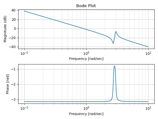
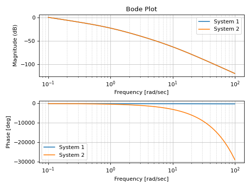
This example shows how the phase is actually computed (with
unwrap=False) and how it is post-processed (withunwrap=True).tf = TransferFunction(1, s**3 + 2*s**2 + s, s) p1 = plot_bode_phase( tf, unwrap=False, show=False, title="unwrap=False") p2 = plot_bode_phase( tf, unwrap=True, show=False, title="unwrap=True") plotgrid(p1, p2)
(
Source code,png)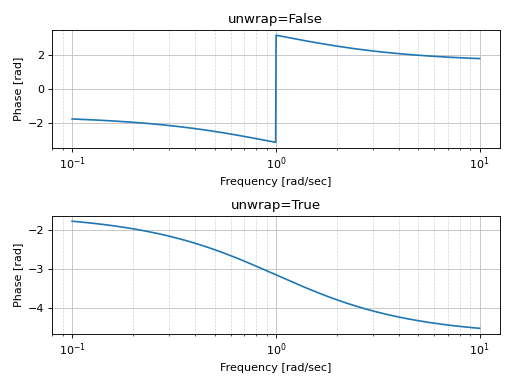
plot_bodealso works with time delays. However, for the post-processing of the phase to work as expected, the frequency range must be sufficiently small, and the number of discretization points must be sufficiently high.from sympy import symbols, exp s = symbols("s") G1 = 1 / (s * (s + 1) * (s + 10)) G2 = G1 * exp(-5*s) plot_bode(G1, G2, phase_unit="deg", n=1e04)
(
Source code,png)
Bode plot of a discrete-time system:
import control as ct
tf = ct.tf([1], [1, 2, 3], dt=0.05)
plot_bode(tf)
(
Source code,png)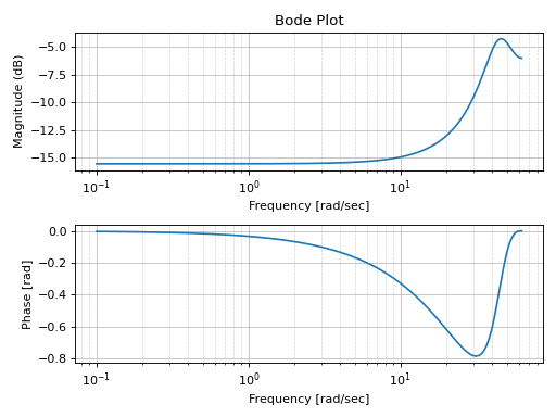
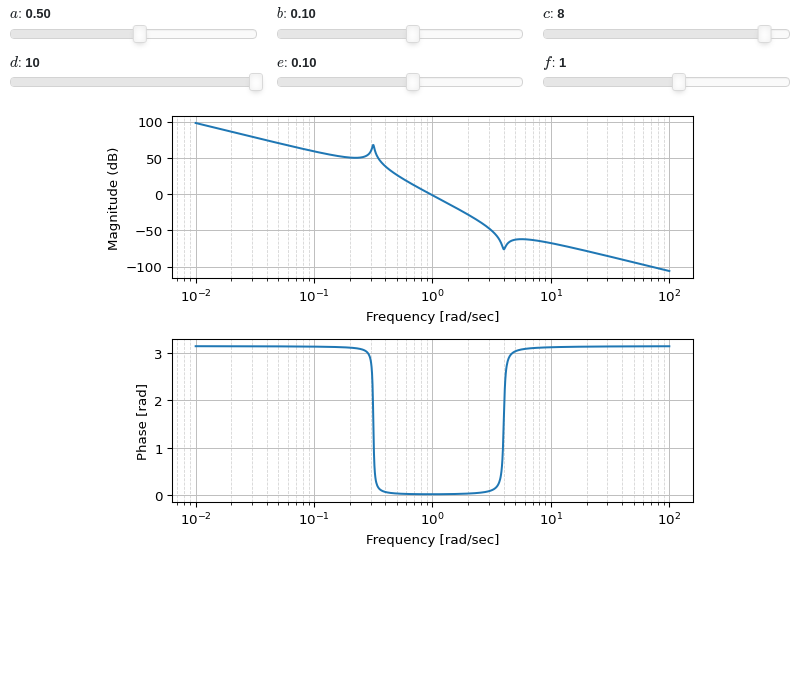
Interactive-widget plot:
from sympy.abc import a, b, c, d, e, f, s
from sympy.physics.control.lti import TransferFunction
from spb import *

tf1 = TransferFunction(a*s**2 + b*s + c, d*s**4 + e*s**3 + f*s**2, s)
plot_bode(
    tf1, initial_exp=-2, final_exp=2,
    params={
        a: (0.5, -10, 10),
        b: (0.1, -1, 1),
        c: (8, -10, 10),
        d: (10, -10, 10),
        e: (0.1, -1, 1),
        f: (1, -10, 10),
    },
    imodule="panel", ncols=3
)
- spb.plot_functions.control.plot_nyquist(*systems, **kwargs)[source]
Plots a Nyquist plot for the system over a (optional) frequency range. The curve is computed by evaluating the Nyquist segment along the positive imaginary axis, with a mirror image generated to reflect the negative imaginary axis. Poles on or near the imaginary axis are avoided using a small indentation. The portion of the Nyquist contour at infinity is not explicitly computed (since it maps to a constant value for any system with a proper transfer function).
- Parameters:
- systemsLTI system type
The LTI system for which the ramp response is to be computed. It can be:
an instance of
sympy.physics.control.lti.TransferFunctionorsympy.physics.control.lti.TransferFunctionMatrixan instance of
control.TransferFunctionan instance of
scipy.signal.TransferFunctiona symbolic expression in rational form, which will be converted to an object of type
sympy.physics.control.lti.TransferFunction.a tuple of two or three elements:
(num, den, generator [opt]), which will be converted to an object of typesympy.physics.control.lti.TransferFunction.a sequence of LTI systems.
a sequence of 2-tuples
(LTI system, label).a dict mapping LTI systems to labels.
- labelstr, optional
The label to be shown on the legend.
- arrowsint or 1D/2D array of floats, optional
Specify the number of arrows to plot on the Nyquist curve. If an integer is passed, that number of equally spaced arrows will be plotted on each of the primary segment and the mirror image. If a 1D array is passed, it should consist of a sorted list of floats between 0 and 1, indicating the location along the curve to plot an arrow.
- max_curve_magnitudefloat, optional
Restrict the maximum magnitude of the Nyquist plot to this value. Portions of the Nyquist plot whose magnitude is restricted are plotted using a different line style.
- max_curve_offsetfloat, optional
When plotting scaled portion of the Nyquist plot, increase/decrease the magnitude by this fraction of the max_curve_magnitude to allow any overlaps between the primary and mirror curves to be avoided.
- mirror_style[str, str] or [dict, dict] or dict or False, optional
Linestyles for mirror image of the Nyquist curve. If a list is given, the first element is used for unscaled portions of the Nyquist curve, the second element is used for portions that are scaled (using max_curve_magnitude). dict is a dictionary of keyword arguments to be passed to the plotting function, for example to plt.plot. If False then omit completely. Default linestyle is [’–’, ‘:’].
- m_circlesbool or float or iterable, optional
Turn on/off M-circles, which are circles of constant closed loop magnitude. If float or iterable (of floats), represents specific magnitudes in dB.
- primary_style[str, str] or [dict, dict] or dict, optional
Linestyles for primary image of the Nyquist curve. If a list is given, the first element is used for unscaled portions of the Nyquist curve, the second element is used for portions that are scaled (using max_curve_magnitude). dict is a dictionary of keyword arguments to be passed to the plotting function, for example to Matplotlib’s plt.plot. Default linestyle is [‘-’, ‘-.’].
- omega_limitsarray_like of two values, optional
Limits to the range of frequencies.
- start_markerstr or dict, optional
Marker to use to mark the starting point of the Nyquist plot. If dict is provided, it must containts keyword arguments to be passed to the plot function, for example to Matplotlib’s plt.plot.
- control_kwdict, optional
A dictionary of keyword arguments passed to
control.nyquist_plot()- **kwargsdict
Refer to
nyquist()for a full list of keyword arguments to customize the appearances of lines.Refer to
graphics()for a full list of keyword arguments to customize the appearances of the figure (title, axis labels, …).
See also
Notes
If a continuous-time system contains poles on or near the imaginary axis, a small indentation will be used to avoid the pole. The radius of the indentation is given by indent_radius and it is taken to the right of stable poles and the left of unstable poles. If a pole is exactly on the imaginary axis, the indent_direction parameter can be used to set the direction of indentation. Setting indent_direction to none will turn off indentation. If return_contour is True, the exact contour used for evaluation is returned.
For those portions of the Nyquist plot in which the contour is indented to avoid poles, resuling in a scaling of the Nyquist plot, the line styles are according to the settings of the primary_style and mirror_style keywords. By default the scaled portions of the primary curve use a dotted line style and the scaled portion of the mirror image use a dashdot line style.
References
Examples
Plotting a single transfer function:
from sympy import Rational
from sympy.abc import s
from sympy.physics.control.lti import TransferFunction
from spb import plot_nyquist
tf1 = TransferFunction(
    4 * s**2 + 5 * s + 1, 3 * s**2 + 2 * s + 5, s)
plot_nyquist(tf1)
(
Source code,png)
Plotting multiple transfer functions and visualizing M-circles:
tf2 = TransferFunction(1, s + Rational(1, 3), s)
plot_nyquist(tf1, tf2,
    m_circles=[-20, -10, -6, -4, -2, 0])
(
Source code,png)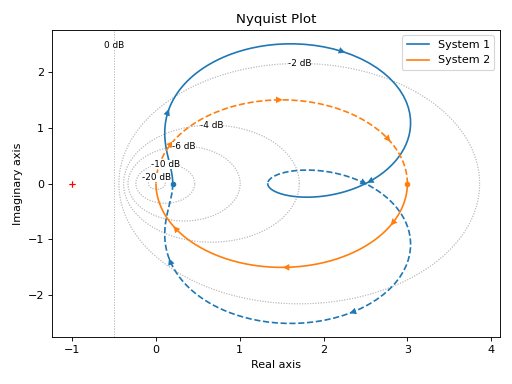
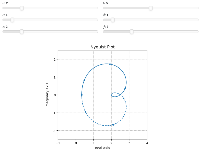
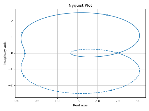
Interactive-widgets plot of a systems:
from sympy.abc import a, b, c, d, e, f, s
from sympy.physics.control.lti import TransferFunction
from spb import plot_nyquist
tf = TransferFunction(a * s**2 + b * s + c, d**2 * s**2 + e * s + f, s)
plot_nyquist(
    tf,
    params={
        a: (2, 0, 10),
        b: (5, 0, 10),
        c: (1, 0, 10),
        d: (1, 0, 10),
        e: (2, 0, 10),
        f: (3, 0, 10),
    },
    m_circles=False,
    xlim=(-1, 4), ylim=(-2.5, 2.5), aspect="equal"
)
- spb.plot_functions.control.plot_nichols(*systems, **kwargs)[source]
Nichols plot for a system over a (optional) frequency range.
- Parameters:
- systemsLTI system type
The LTI system for which the ramp response is to be computed. It can be:
an instance of
sympy.physics.control.lti.TransferFunctionorsympy.physics.control.lti.TransferFunctionMatrixan instance of
control.TransferFunctionan instance of
scipy.signal.TransferFunctiona symbolic expression in rational form, which will be converted to an object of type
sympy.physics.control.lti.TransferFunction.a tuple of two or three elements:
(num, den, generator [opt]), which will be converted to an object of typesympy.physics.control.lti.TransferFunction.a sequence of LTI systems.
a sequence of 2-tuples
(LTI system, label).a dict mapping LTI systems to labels.
- ngridbool, optional
Turn on/off the [Nichols] grid lines.
- omega_limitsarray_like of two values, optional
Limits to the range of frequencies.
- **kwargsdict
Refer to
nichols()for a full list of keyword arguments to customize the appearances of lines.Refer to
graphics()for a full list of keyword arguments to customize the appearances of the figure (title, axis labels, …).
See also
References
Examples
Plotting a single transfer function:
from sympy.abc import s
from sympy.physics.control.lti import TransferFunction
from spb import plot_nichols
tf = TransferFunction(50*s**2 - 20*s + 15, -10*s**2 + 40*s + 30, s)
plot_nichols(tf)
(
Source code,png)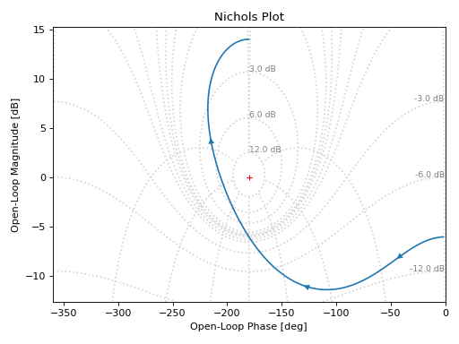
Turning off the Nichols grid lines:
plot_nichols(tf, ngrid=False)
(
Source code,png)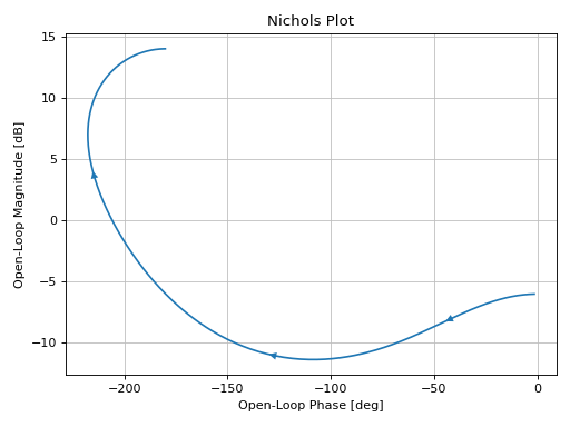
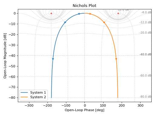
Plotting multiple transfer functions:
tf1 = TransferFunction(1, s**2 + 2*s + 1, s)
tf2 = TransferFunction(1, s**2 - 2*s + 1, s)
plot_nichols(tf1, tf2, xlim=(-360, 360))
(
Source code,png)
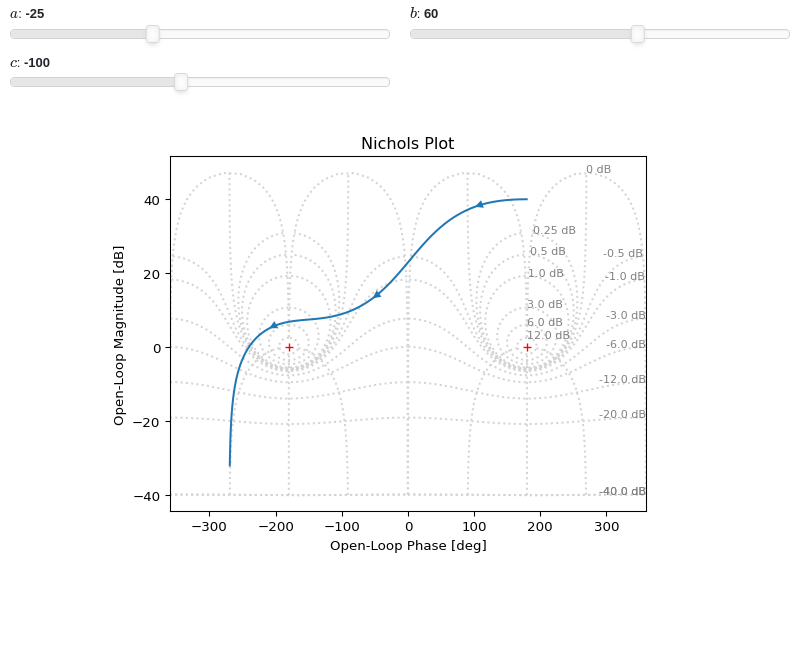
Interactive-widgets plot of a systems. For these kind of plots, it is recommended to set both
omega_limitsandxlim:from sympy.abc import a, b, c, s from spb import plot_nichols from sympy.physics.control.lti import TransferFunction tf = TransferFunction(a*s**2 + b*s + c, s**3 + 10*s**2 + 5 * s + 1, s) plot_nichols( tf, omega_limits=[1e-03, 1e03], n=1e04, params={ a: (-25, -100, 100), b: (60, -300, 300), c: (-100, -1000, 1000), }, xlim=(-360, 360) )

- spb.plot_functions.control.plot_root_locus(*systems, sgrid=True, zgrid=False, **kwargs)[source]
Root Locus plot for one or multiple systems.
- Parameters:
- systemsLTI system type
The LTI system for which the ramp response is to be computed. It can be:
an instance of
sympy.physics.control.lti.TransferFunctionorsympy.physics.control.lti.TransferFunctionMatrixan instance of
control.TransferFunctionan instance of
scipy.signal.TransferFunctiona symbolic expression in rational form, which will be converted to an object of type
sympy.physics.control.lti.TransferFunction.a tuple of two or three elements:
(num, den, generator [opt]), which will be converted to an object of typesympy.physics.control.lti.TransferFunction.a sequence of LTI systems.
a sequence of 2-tuples
(LTI system, label).a dict mapping LTI systems to labels.
- labelstr, optional
The label to be shown on the legend.
- rendering_kwdict, optional
A dictionary of keywords/values which is passed to the backend’s function to customize the appearance of lines. Refer to the plotting library (backend) manual for more informations.
- control_kwdict
A dictionary of keyword arguments to be passed to
control.root_locus().- sgridbool, optional
Generates a grid of constant damping ratios and natural frequencies on the s-plane. Default to True.
- zgridbool, optional
Generates a grid of constant damping ratios and natural frequencies on the z-plane. Default to False. If
zgrid=True, then it will automatically setssgrid=False.- inputint, optional
Only compute the poles/zeros for the listed input. If not specified, the poles/zeros for each independent input are computed (as separate traces).
- outputint, optional
Only compute the poles/zeros for the listed output. If not specified, all outputs are reported.
- **kwargs
Keyword arguments are the same as
line(). Refer to its documentation for a for a full list of keyword arguments.
Notes
This function uses the
python-controlmodule to generate the numerical data.Examples
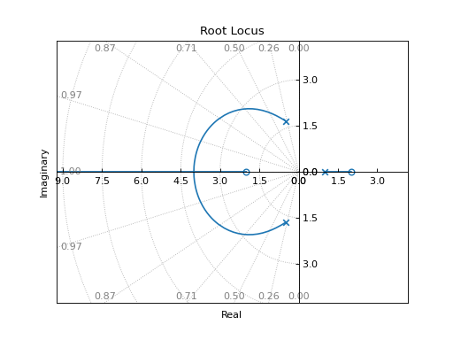
Plotting a single transfer function on the s-plane:
from sympy.abc import s, z
from spb import plot_root_locus
G1 = (s**2 - 4) / (s**3 + 2*s - 3)
plot_root_locus(G1)
(
Source code,png)
Plotting a discrete transfer function on the z-plane:
G2 = (0.038*z + 0.031)/(9.11*z**2 - 13.77*z + 5.0)
plot_root_locus(G2, zgrid=True, aspect="equal")
(
Source code,png)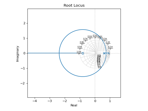
Plotting multiple transfer functions:
from sympy.abc import s
from spb import plot_root_locus
G3 = (s**2 + 1) / (s**3 + 2*s**2 + 3*s + 4)
plot_root_locus(G1, G3)
(
Source code,png)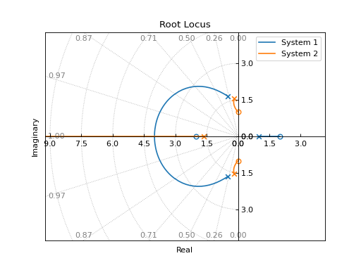
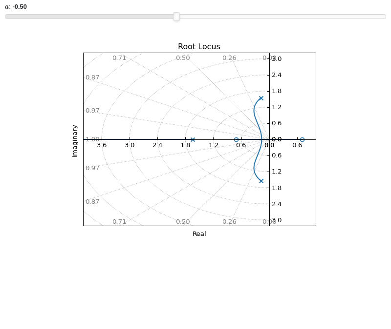
Interactive-widgets root locus plot:
from sympy import symbols
from spb import *
a, s = symbols("a, s")
G = (s**2 + a) / (s**3 + 2*s**2 + 3*s + 4)
params={a: (-0.5, -4, 4)}
plot_root_locus(G, params=params, xlim=(-4, 1))
