Vectors
NOTE:
For technical reasons, all interactive-widgets plots in this documentation
are created using Holoviz’s Panel. Often, they will ran just fine with
ipywidgets too. However, if a specific example uses the param library,
or widgets from the panel module, then users will have to modify the
params dictionary in order to make it work with ipywidgets.
Refer to Interactive module for more information.
- spb.plot_functions.vectors.plot_vector(*args, **kwargs)[source]
Plot a 2D or 3D vector field. By default, the aspect ratio of the plot is set to aspect=”equal”.
Typical usage examples are in the followings:
Plotting a 2D vector field:
plot_vector(vec, range_x, range_y, **kwargs)
Plotting multiple 2D vector fields with different ranges and custom labels:
plot_vector(
   (vec1, range1_x, range1_y, label1 [opt]),
   (vec2, range2_x, range2_y, label2 [opt]),
   **kwargs)
Plotting a 3D vector field:
plot_vector(vec, range_x, range_y, range_z, **kwargs)
Plotting multiple 3D vector fields with different ranges and custom labels:
plot_vector(
   (vec1, range1_x, range1_y, range1_z, label1 [opt]),
   (vec2, range2_x, range2_y, range2_z, label2 [opt]),
   **kwargs)
Refer to
vector_field_2d()for a full list of keyword arguments to customize the appearances of quivers, streamlines and contours for a 2D vector field.Refer to
vector_field_3d()for a full list of keyword arguments to customize the appearances of quivers and streamlines for a 3D vector field.Refer to
graphics()for a full list of keyword arguments to customize the appearances of the figure (title, axis labels, …).Examples
>>> from sympy import symbols, sin, cos, Plane, Matrix, sqrt, latex
>>> from spb import plot_vector
>>> x, y, z = symbols('x, y, z')
Quivers plot of a 2D vector field with a contour plot in background representing the vector’s magnitude (a scalar field).
>>> v = [sin(x - y), cos(x + y)]
>>> plot_vector(v, (x, -3, 3), (y, -3, 3),
...     quiver_kw=dict(color="black", scale=30, headwidth=5),
...     contour_kw={"cmap": "Blues_r", "levels": 15},
...     grid=False, xlabel="x", ylabel="y")
Plot object containing:
[0]: contour: sqrt(sin(x - y)**2 + cos(x + y)**2) for x over (-3, 3) and y over (-3, 3)
[1]: 2D vector series: [sin(x - y), cos(x + y)] over (x, -3.0, 3.0), (y, -3.0, 3.0)
(
Source code,png)
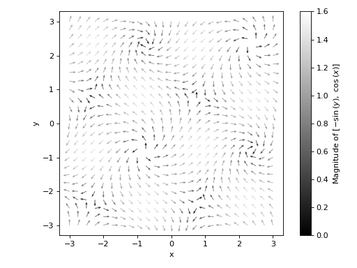
Quivers plot of a 2D vector field with no background scalar field, a custom label and normalized quiver lengths:
>>> plot_vector(
...     v, (x, -3, 3), (y, -3, 3),
...     label="Magnitude of $%s$" % latex([-sin(y), cos(x)]),
...     scalar=False, normalize=True,
...     quiver_kw={
...         "scale": 35, "headwidth": 4, "cmap": "gray",
...         "clim": [0, 1.6]},
...     grid=False, xlabel="x", ylabel="y")
Plot object containing:
[0]: 2D vector series: [sin(x - y), cos(x + y)] over (x, -3.0, 3.0), (y, -3.0, 3.0)
(
Source code,png)
Streamlines plot of a 2D vector field with no background scalar field, and a custom label:
>>> plot_vector(v, (x, -3, 3), (y, -3, 3),
...     streamlines=True, scalar=None,
...     stream_kw={"density": 1.5},
...     label="Magnitude of %s" % str(v), xlabel="x", ylabel="y")
Plot object containing:
[0]: 2D vector series: [sin(x - y), cos(x + y)] over (x, -3.0, 3.0), (y, -3.0, 3.0)
(
Source code,png)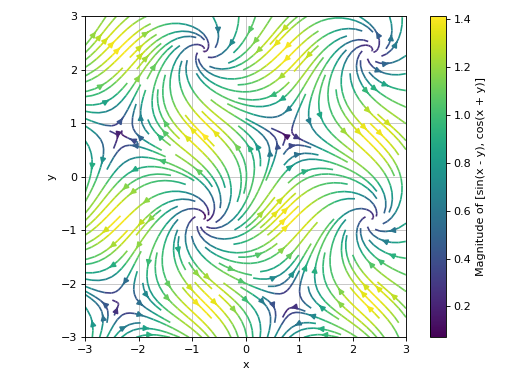
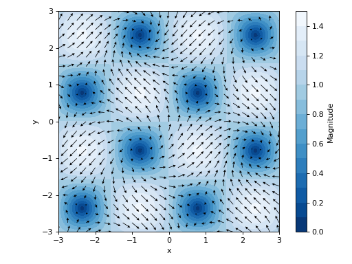
Plot multiple 2D vectors fields, setting a background scalar field to be the magnitude of the first vector. Also, apply custom rendering options to all data series.
>>> scalar_expr = sqrt((-sin(y))**2 + cos(x)**2)
>>> plot_vector([-sin(y), cos(x)], [2 * y, x], (x, -5, 5), (y, -3, 3),
...     n=20, legend=True, grid=False, xlabel="x", ylabel="y",
...     scalar=[scalar_expr, "$%s$" % latex(scalar_expr)], use_cm=False,
...     rendering_kw=[
...         {"cmap": "summer"}, # to the contour
...         {"color": "k"},     # to the first quiver
...         {"color": "r"}      # to the second quiver
... ])
Plot object containing:
[0]: contour: sqrt(sin(y)**2 + cos(x)**2) for x over (-5, 5) and y over (-3, 3)
[1]: 2D vector series: [-sin(y), cos(x)] over (x, -5.0, 5.0), (y, -3.0, 3.0)
[2]: 2D vector series: [2*y, x] over (x, -5.0, 5.0), (y, -3.0, 3.0)
(
Source code,png)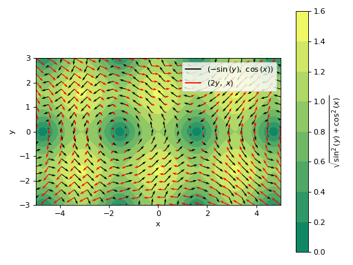
Plotting a the streamlines of a 2D vector field defined with numerical functions instead of symbolic expressions:
>>> import numpy as np
>>> f = lambda x, y: np.sin(2 * x + 2 * y)
>>> fx = lambda x, y: np.cos(f(x, y))
>>> fy = lambda x, y: np.sin(f(x, y))
>>> plot_vector([fx, fy], ("x", -1, 1), ("y", -1, 1),
...     streamlines=True, scalar=False, use_cm=False)
(
Source code,png)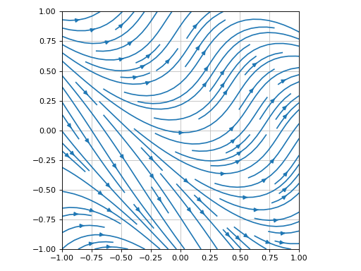
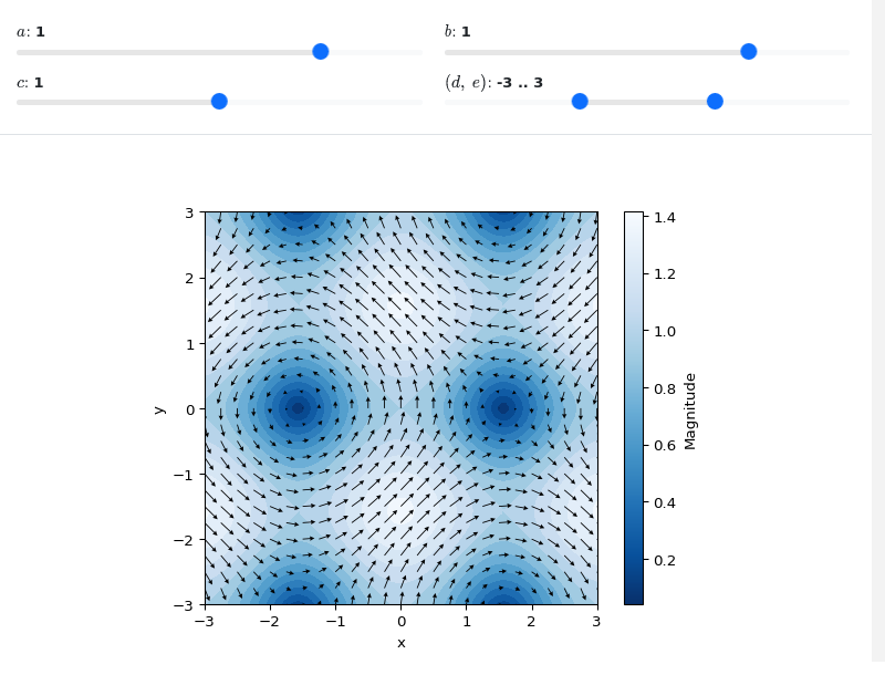
Interactive-widget 2D vector plot. Refer to the interactive sub-module documentation to learn more about the
paramsdictionary. This plot illustrates:customizing the appearance of quivers and countour.
the use of
prange(parametric plotting range).the use of the
paramsdictionary to specify sliders in their basic form: (default, min, max).the use of
panel.widgets.slider.RangeSlider, which is a 2-values widget.
from sympy import *
from spb import *
import panel as pn
x, y, a, b, c, d, e = symbols("x, y, a, b, c, d, e")
v = [-sin(a * y), cos(b * x)]
plot_vector(
    v, prange(x, -3*c, 3*c), prange(y, d, e),
    params={
        a: (1, -2, 2), b: (1, -2, 2),
        c: (1, 0, 2),
        (d, e): pn.widgets.RangeSlider(
            value=(-3, 3), start=-9, end=9, step=0.1)
    },
    quiver_kw=dict(color="black", scale=30, headwidth=5),
    contour_kw={"cmap": "Blues_r", "levels": 15},
    grid=False, xlabel="x", ylabel="y",
    imodule="panel", servable=True
)
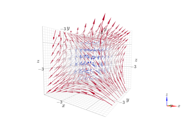
3D vector field.
from sympy import *
from spb import *
var("x:z")
plot_vector([z, y, x], (x, -10, 10), (y, -10, 10), (z, -10, 10),
    backend=KB, n=8, xlabel="x", ylabel="y", zlabel="z",
    quiver_kw={"scale": 0.5, "line_width": 0.1, "head_size": 10})
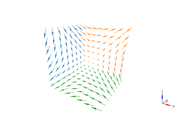
3D vector field with 3 orthogonal slice planes.
from sympy import *
from spb import *
var("x:z")
plot_vector([z, y, x], (x, -10, 10), (y, -10, 10), (z, -10, 10),
    backend=KB, n=8, use_cm=False, grid=False,
    xlabel="x", ylabel="y", zlabel="z",
    quiver_kw={"scale": 0.25, "line_width": 0.1, "head_size": 10},
    slice=[
        Plane((-10, 0, 0), (1, 0, 0)),
        Plane((0, 10, 0), (0, 2, 0)),
        Plane((0, 0, -10), (0, 0, 1))])
3D vector streamlines starting at a 300 random points:
from sympy import *
from spb import *
import k3d
var("x:z")
plot_vector(Matrix([z, -x, y]), (x, -3, 3), (y, -3, 3), (z, -3, 3),
    backend=KB, n=40, streamlines=True,
    stream_kw=dict(
        starts=True,
        npoints=400,
        width=0.025,
        color_map=k3d.colormaps.matplotlib_color_maps.viridis
    ),
    xlabel="x", ylabel="y", zlabel="z")

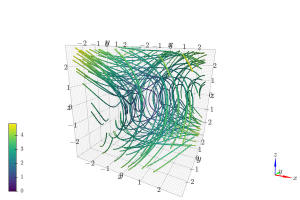
3D vector streamlines starting at the XY plane. Note that the number of discretization points of the plane controls the numbers of streamlines.
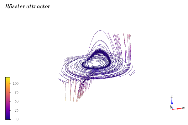
from sympy import *
from spb import *
import k3d
var("x:z")
u = -y - z
v = x + y / 5
w = S(1) / 5 + (x - S(5) / 2) * z
s = 10 # length of the cubic discretization volume
# create an XY plane with n discretization points along each direction
n = 8
p1 = plot_geometry(
    Plane((0, 0, 0), (0, 0, 1)), (x, -s, s), (y, -s, s), (z, -s, s),
    n1=n, n2=n, show=False)
# extract the coordinates of the starting points for the streamlines
xx, yy, zz = p1[0].get_data()
# streamlines plot
plot_vector(Matrix([u, v, w]), (x, -s, s), (y, -s, s), (z, -s, s),
    backend=KB, n=40, streamlines=True, grid=False,
    stream_kw=dict(
        starts=dict(x=xx, y=yy, z=zz),
        width=0.025,
        color_map=k3d.colormaps.matplotlib_color_maps.plasma
    ),
    title="Rössler \, attractor", xlabel="x", ylabel="y", zlabel="z")

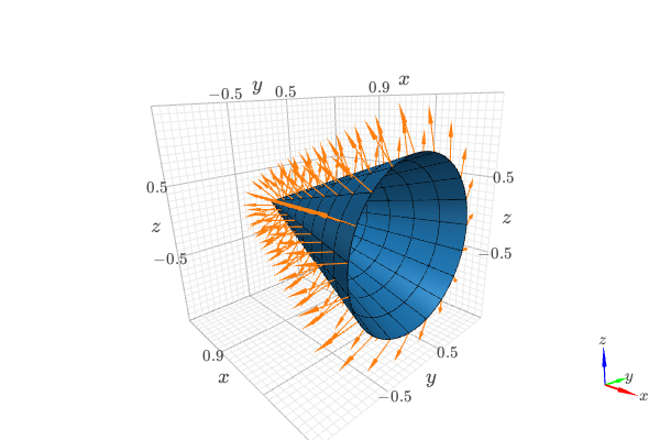
Visually verify the normal vector to a circular cone surface. The following steps are executed:
compute the normal vector to a circular cone surface. This will be the vector field to be plotted.
plot the cone surface for visualization purposes (use high number of discretization points).
plot the cone surface that will be used to slice the vector field (use a low number of discretization points). The data series associated to this plot will be used in the
slicekeyword argument in the next step.plot the sliced vector field.
combine the plots of step 4 and 2 to get a nice visualization.
from sympy import tan, cos, sin, pi, symbols
from spb import plot3d_parametric_surface, plot_vector, KB
from sympy.vector import CoordSys3D, gradient

u, v = symbols("u, v")
N = CoordSys3D("N")
i, j, k = N.base_vectors()
xn, yn, zn = N.base_scalars()

t = 0.35    # half-cone angle in radians
expr = -xn**2 * tan(t)**2 + yn**2 + zn**2    # cone surface equation
g = gradient(expr)
n = g / g.magnitude()    # unit normal vector
n1, n2 = 10, 20 # number of discretization points for the vector field

# cone surface for visualization (high number of discretization points)
p1 = plot3d_parametric_surface(
    u / tan(t), u * cos(v), u * sin(v), (u, 0, 1), (v, 0 , 2*pi),
    {"opacity": 1}, backend=KB, show=False, wireframe=True,
    wf_n1=n1, wf_n2=n2, wf_rendering_kw={"width": 0.004})
# cone surface to discretize vector field (low numb of discret points)
p2 = plot3d_parametric_surface(
    u / tan(t), u * cos(v), u * sin(v), (u, 0, 1), (v, 0 , 2*pi),
    n1=n1, n2=n2, show=False)
# plot vector field on over the surface of the cone
p3 = plot_vector(
    n, (xn, -5, 5), (yn, -5, 5), (zn, -5, 5), slice=p2[0],
    backend=KB, use_cm=False, show=False,
    quiver_kw={"scale": 0.5, "pivot": "tail"})
(p1 + p3).show()
