Complex Analysis

NOTE: For technical reasons, all interactive-widgets plots in this documentation are created using Holoviz’s Panel. Often, they will ran just fine with ipywidgets too. However, if a specific example uses the param library, or widgets from the panel module, then users will have to modify the params dictionary in order to make it work with ipywidgets. Refer to Interactive module for more information.

spb.plot_functions.complex_analysis.plot_complex(*args, **kwargs)

Plot the absolute value of a complex function colored by its argument. By default, the aspect ratio of 2D plots is set to aspect="equal".

Depending on the provided range, this function will produce different types of plots:

1. Line plot over the reals.

2. Image plot over the complex plane if threed=False. This is also known as Domain Coloring. Use the coloring keyword argument to select a different coloring strategy and cmap to set a custom color map (default to HSV).

3. If threed=True, plot a 3D surface of the absolute value over the complex plane, colored by its argument. Use the coloring keyword argument to select a different coloring strategy and cmap to set a custom color map (default to HSV).

Typical usage examples are in the followings:

• Plotting a single expression with a single range:

  plot_complex(expr, range, **kwargs)
  

• Plotting multiple expressions with different ranges, custom labels and rendering options:

  plot_complex(
     (expr1, range1, label1 [opt], rendering_kw1 [opt]),
     (expr2, range2, label2 [opt], rendering_kw2 [opt]),
     ..., **kwargs)
  

Refer to line_abs_arg_colored() or domain_coloring() or analytic_landscape() for a full list of keyword arguments to customize the appearances of lines and surfaces.

Refer to graphics() for a full list of keyword arguments to customize the appearances of the figure (title, axis labels, …).

See also

plot_riemann_sphere, plot_real_imag, plot_complex_list

plot_complex_vector

Examples

>>> from sympy import I, symbols, exp, sqrt, cos, sin, pi, gamma
>>> from spb import plot_complex
>>> x, y, z = symbols('x, y, z')

(Source code)

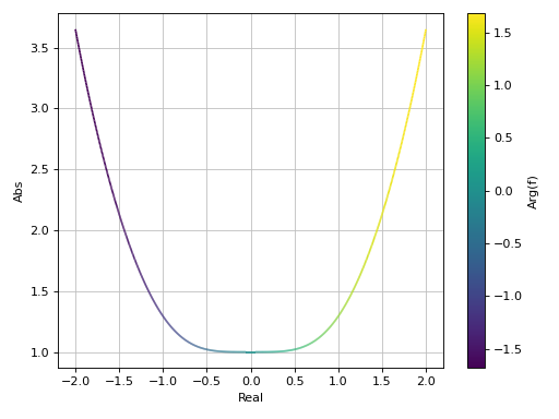
Plot the modulus of a complex function colored by its magnitude:

>>> plot_complex(cos(x) + sin(I * x), "f", (x, -2, 2))
Plot object containing:
[0]: cartesian abs-arg line: cos(x) + I*sinh(x) for x over ((-2+0j), (2+0j))

(Source code, png)

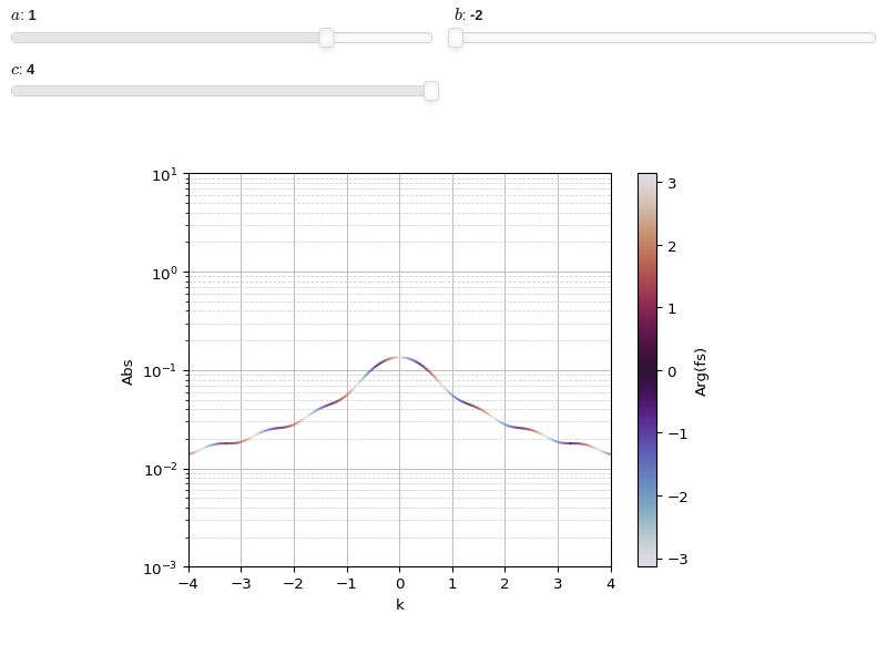
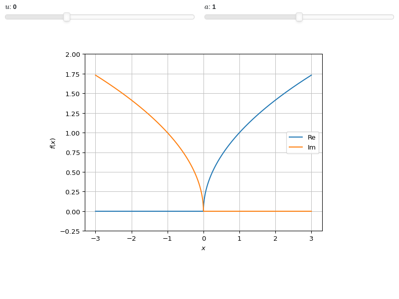
Interactive-widget plot of a Fourier Transform. Refer to the interactive sub-module documentation to learn more about the params dictionary. This plot illustrates:

• the use of prange (parametric plotting range).

• for plot_complex, symbols going into prange must be real.

• the use of the params dictionary to specify sliders in their basic form: (default, min, max).

from sympy import *
from spb import *
x, k, a, b = symbols("x, k, a, b")
c = symbols("c", real=True)
f = exp(-x**2) * (Heaviside(x + a) - Heaviside(x - b))
fs = fourier_transform(f, x, k)
plot_complex(fs, prange(k, -c, c),
        params={a: (1, -2, 2), b: (-2, -2, 2), c: (4, 0.5, 4)},
        label="Arg(fs)", xlabel="k", yscale="log", ylim=(1e-03, 10))

(Source code, small.png)

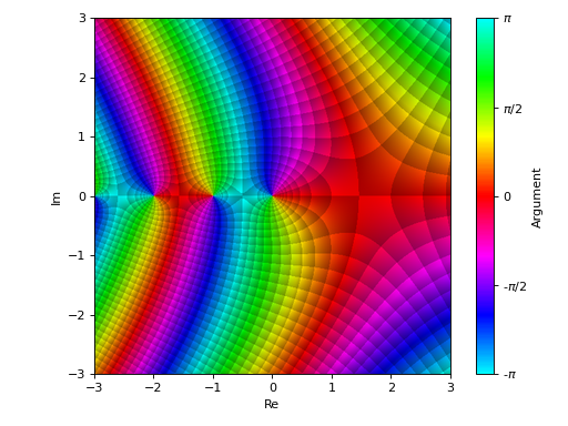
Domain coloring plot. To improve the smoothness of the results, increase the number of discretization points and/or apply an interpolation (if the backend supports it):

>>> plot_complex(gamma(z), (z, -3-3j, 3+3j),
...     coloring="b", n=500, grid=False)
Plot object containing:
[0]: complex domain coloring: gamma(z) for re(z) over (-3.0, 3.0) and im(z) over (-3.0, 3.0)

(Source code, png)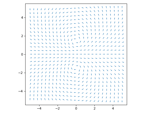

Domain coloring of the same function evaluated near the point \(z=\infty\):

>>> plot_complex(gamma(z), (z, -1-1j, 1+1j), coloring="b", n=500,
...     grid=False, at_infinity=True, axis=False)
Plot object containing:
[0]: complex domain coloring: gamma(1/z) for re(z) over (-1.0, 1.0) and im(z) over (-1.0, 1.0)

(Source code, png)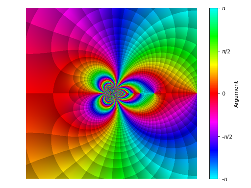

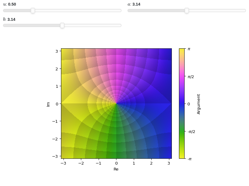
Interactive-widget domain coloring plot. Refer to the interactive sub-module documentation to learn more about the params dictionary. This plot illustrates:

• setting a custom colormap and adjusting the black-level of the enhanced visualization.

• the use of prange (parametric plotting range).

• the use of the params dictionary to specify sliders in their basic form: (default, min, max).

from sympy import *
from spb import *
import colorcet
z, u, a, b = symbols("z, u, a, b")
plot_complex(
    sin(u * z), prange(z, -a - b*I, a + b*I),
    cmap=colorcet.colorwheel, blevel=0.85,
    coloring="b", n=250, grid=False,
    params={
        u: (0.5, 0, 2),
        a: (pi, 0, 2*pi),
        b: (pi, 0, 2*pi),
    })

(Source code, small.png)

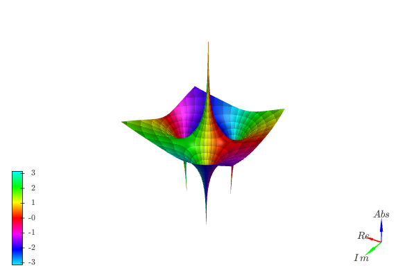
The analytic landscape is 3D plot of the absolute value of a complex function colored by its argument:

from sympy import symbols, gamma, I
from spb import plot_complex, PB
z = symbols('z')
plot_complex(gamma(z), (z, -3 - 3*I, 3 + 3*I), threed=True,
    backend=PB, zlim=(-1, 6), use_cm=True)

(Source code, png)

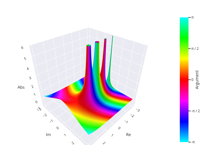
Because the function goes to infinity at poles, sometimes it might be beneficial to visualize the logarithm of the absolute value in order to easily identify zeros:

from sympy import symbols, I
from spb import plot_complex, KB
z = symbols("z")
expr = (z**3 - 5) / z
plot_complex(expr, (z, -3-3j, 3+3j), coloring="b", threed=True,
    use_cm=True, grid=False, n=500, backend=KB, tz=np.log)

(Source code, small.png)

spb.plot_functions.complex_analysis.plot_riemann_sphere(expr, range=None, annotate=True, riemann_mask=True, **kwargs)

Visualize stereographic projections of the Riemann sphere.

Note:

1. Differently from other plot functions that return instances of BaseBackend, this function returns a Matplotlib figure.

2. This function calls plot_complex(): refer to its documentation for the full list of keyword arguments.

Parameters:

args

exprExpr

Represent the complex function to be plotted.

range3-element tuple, optional

Denotes the range of the variables. Only works for 2D plots. Default to (z, -1.25 - 1.25*I, 1.25 + 1.25*I).

annotateboolean, optional

Turn on/off the annotations on the 2D projections of the Riemann sphere. Default to True (annotations are visible). They can only be visible when riemann_mask=True.

riemann_maskboolean, optional

Turn on/off the unit disk mask representing the Riemann sphere on the 2D projections. Default to True (mask is active).

axisboolean, optional

Turn on/off the axis of the 2D subplots. Default to False (axis not visible).

size(width, height)

Specify the size of the resulting figure.

titlestr, list, optional

A list of two strings representing the titles for the two plots.

See also

plot_complex

Notes

The [Riemann-sphere] is a model of the extented complex plane, comprised of the complex plane plus a point at infinity. Let’s consider a 3D space with a sphere of radius 1 centered at the origin. The xy plane, representing the complex plane, cut the sphere in half at the equator. The [Stereographic] projection of any point in the complex plane on the sphere is given by the intersection point between a line connecting the complex point with the north pole of the sphere. Let’s consider the magnitude of a complex point:

• if its lower than one (points inside the unit disk), then the point is mapped to the Southern Hemisphere (the line connecting the complex point to the north pole intersects the sphere in the Southern Hemisphere). The origin of the complex plane is mapped to the south pole.

• if its equal to one (points in the unit circle), then the point is already on the sphere, specifically in its equator.

• if its greater than one (point outside the unit disk), then the point is mapped to the Northen Hemisphere. The north pole represents the point at infinity.

Visualizing a 3D sphere is difficult (refer to [Wegert] for more information): the most obvious problem is that only a part can be seen from any location. A better way to fully visualize the sphere is with two 2D charts depicting the sphere from the inside:

1. a stereographic projection of the sphere from the north pole, which depict the Southern Hemisphere. It corresponds to an ordinary (enhanced) domain coloring plot around the complex point \(z=0\).

2. a stereographic projection of the sphere from the south pole, which depict the Northen Hemisphere. It corresponds to an ordinary (enhanced) domain coloring plot around the complex point \(z=\infty\) (infinity). Practically, it depicts the transformation \(z \rightarrow \frac{1}{z}\).

Let’s look at an example:

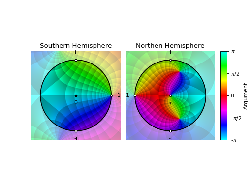
from sympy import symbols, pi
from spb import *
z = symbols("z")
expr = (z - 1) / (z**2 + z + 2)
plot_riemann_sphere(expr, coloring="b", n=800)

(Source code, png)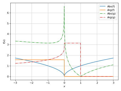

The saturated disks represents the hemispheres. The black circle is the equator. Also, a few important points are displayed to make the plot easier to understand.

Note the orientation of the Northen Hemisphere: it has been rotated around the point at infinity by an angle pi and flipped about the real axis. This is convenient because:

1. we can now imagine to fold the two charts so that the points 1, i, -i are overlayed, glue the equator and blow it up to obtain a sphere.

2. imagine bringing the two discs closer so that they touch at the point 1. Now, roll the two discs together: assuming there are no branch cuts, there is continuity of argument and absolute value across the equator: what is outside of the disc in the left plot, is inside of the disk in the second plot, and vice-versa.

From the above plots, the zero located at \(z=1\) is clearly visible, as well as the two poles located at \(z = -\frac{1}{2} - i \frac{\sqrt{7}}{2}\) and \(z = -\frac{1}{2} + i \frac{\sqrt{7}}{2}\). Not obvious at first, there is a zero located at \(z=\infty\). We can tell its a zero by looking at ordering of colors around it in comparison to the poles. Alternatively, we can use some enhanced color scheme, for example one which brings poles to white:

plot_riemann_sphere(expr, coloring="m", n=800)

(Source code, png)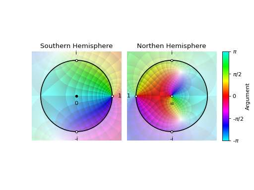

Examples

Standard output:

from sympy import symbols, Rational, I
from spb import *
z = symbols("z")
expr = 1 / (2 * z**2) + z
plot_riemann_sphere(expr, coloring="b", n=800)

(Source code, png)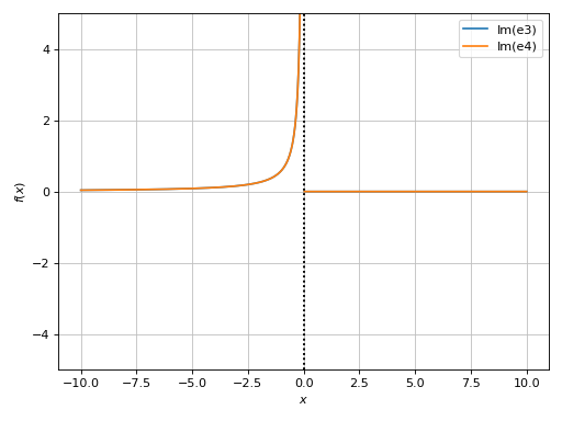

Hide annotations:

plot_riemann_sphere(expr, coloring="b", n=800, annotate=False)

(Source code, png)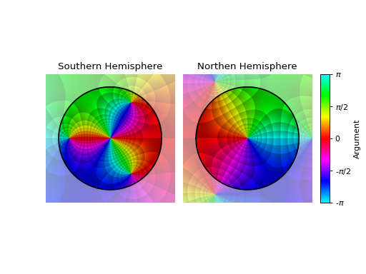

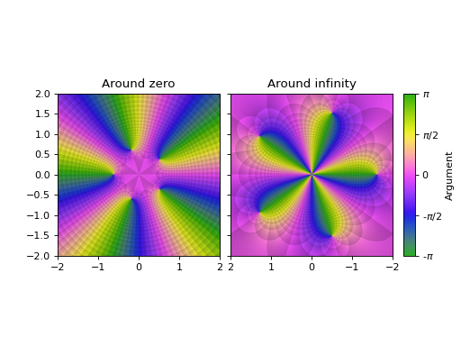
Hiding Riemann disk mask and annotations, set a custom domain, show axis (note that the right-most plot might be misleading because the center represents infinity), custom colormap, set the black level of contours, set titles.

import colorcet
expr = z**5 + Rational(1, 10)
l = 2
plot_riemann_sphere(
    expr, (z, -l-l*I, l+l*I), coloring="b", n=800,
    riemann_mask=False, axis=True, grid=False,
    cmap=colorcet.CET_C2, blevel=0.85,
    title=["Around zero", "Around infinity"])

(Source code, png)

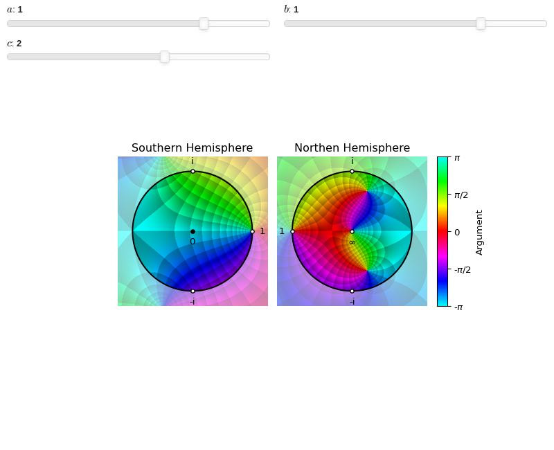
Interactive-widget plot. Refer to the interactive sub-module documentation to learn more about the params dictionary. This plot illustrates the use of the params dictionary to specify sliders in their basic form: (default, min, max).

from sympy import *
from sympy.abc import a, b, c
from spb import *
z = symbols("z")
expr = (z - 1) / (a * z**2 + b * z + c)
plot_riemann_sphere(
    expr, coloring="b", n=300,
    params={
        a: (1, -2, 2),
        b: (1, -2, 2),
        c: (2, -10, 10),
    }
)

(Source code, small.png)

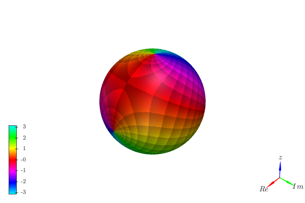
3D plot of a complex function on the Riemann sphere. Note, the higher the number of discretization points, the better the final results, but the higher memory consumption:

from sympy import *
from spb import *
z = symbols("z")
expr = (z - 1) / (z**2 + z + 1)
plot_riemann_sphere(expr, threed=True, n=150,
    coloring="b", backend=KB, legend=False, grid=False)

(Source code, small.png)

spb.plot_functions.complex_analysis.plot_complex_list(*args, **kwargs)

Plot lists of complex points. By default, the aspect ratio of the plot is set to aspect="equal".

Typical usage examples are in the followings:

• Plotting a single list of complex numbers:

  plot_complex_list(l1, **kwargs)
  

• Plotting multiple lists of complex numbers:

  plot_complex_list(l1, l2, **kwargs)
  

• Plotting multiple lists of complex numbers each one with a custom label and rendering options:

  plot_complex_list(
     (l1, label1, rendering_kw1),
     (l2, label2, rendering_kw2), **kwargs)`
  

Refer to complex_points() for a full list of keyword arguments to customize the appearances of lines.

Refer to graphics() for a full list of keyword arguments to customize the appearances of the figure (title, axis labels, …).

See also

plot_real_imag, plot_complex, plot_complex_vector

Examples

>>> from sympy import I, symbols, exp, sqrt, cos, sin, pi, gamma
>>> from spb import plot_complex_list
>>> x, y, z = symbols('x, y, z')

(Source code)

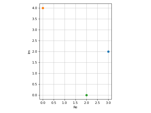
Plot individual complex points:

>>> plot_complex_list(3 + 2 * I, 4 * I, 2)
Plot object containing:
[0]: complex points: (3 + 2*I,)
[1]: complex points: (4*I,)
[2]: complex points: (2,)

(Source code, png)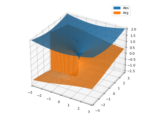

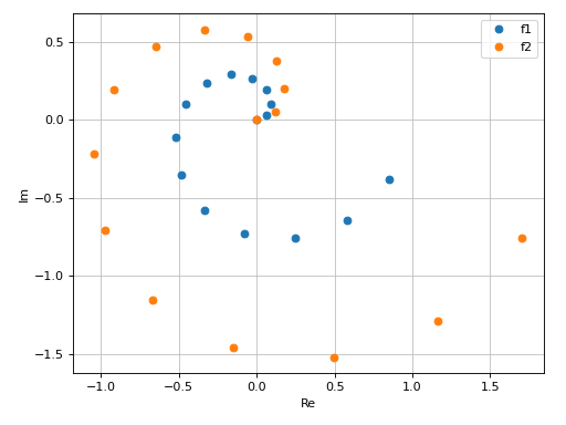
Plot two lists of complex points and assign to them custom labels:

>>> expr1 = z * exp(2 * pi * I * z)
>>> expr2 = 2 * expr1
>>> n = 15
>>> l1 = [expr1.subs(z, t / n) for t in range(n)]
>>> l2 = [expr2.subs(z, t / n) for t in range(n)]
>>> plot_complex_list((l1, "f1"), (l2, "f2"))
Plot object containing:
[0]: complex points: (0.0, 0.0666666666666667*exp(0.133333333333333*I*pi), 0.133333333333333*exp(0.266666666666667*I*pi), 0.2*exp(0.4*I*pi), 0.266666666666667*exp(0.533333333333333*I*pi), 0.333333333333333*exp(0.666666666666667*I*pi), 0.4*exp(0.8*I*pi), 0.466666666666667*exp(0.933333333333333*I*pi), 0.533333333333333*exp(1.06666666666667*I*pi), 0.6*exp(1.2*I*pi), 0.666666666666667*exp(1.33333333333333*I*pi), 0.733333333333333*exp(1.46666666666667*I*pi), 0.8*exp(1.6*I*pi), 0.866666666666667*exp(1.73333333333333*I*pi), 0.933333333333333*exp(1.86666666666667*I*pi))
[1]: complex points: (0, 0.133333333333333*exp(0.133333333333333*I*pi), 0.266666666666667*exp(0.266666666666667*I*pi), 0.4*exp(0.4*I*pi), 0.533333333333333*exp(0.533333333333333*I*pi), 0.666666666666667*exp(0.666666666666667*I*pi), 0.8*exp(0.8*I*pi), 0.933333333333333*exp(0.933333333333333*I*pi), 1.06666666666667*exp(1.06666666666667*I*pi), 1.2*exp(1.2*I*pi), 1.33333333333333*exp(1.33333333333333*I*pi), 1.46666666666667*exp(1.46666666666667*I*pi), 1.6*exp(1.6*I*pi), 1.73333333333333*exp(1.73333333333333*I*pi), 1.86666666666667*exp(1.86666666666667*I*pi))

(Source code, png)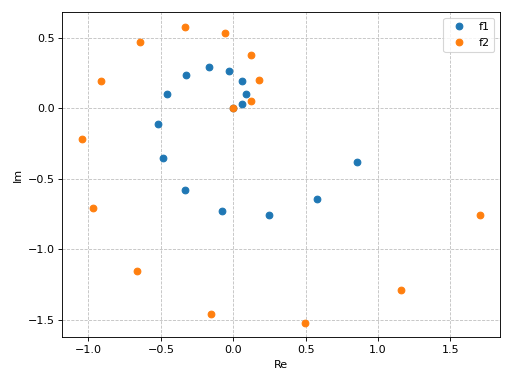

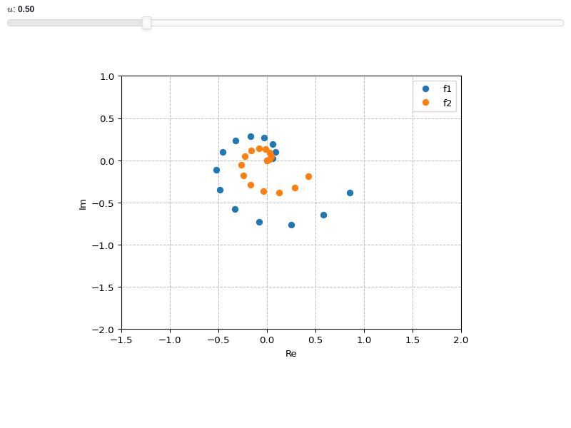
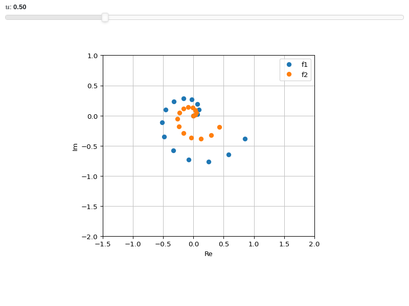
Interactive-widget plot. Refer to the interactive sub-module documentation to learn more about the params dictionary.

from sympy import *
from spb import *
z, u = symbols("z u")
expr1 = z * exp(2 * pi * I * z)
expr2 = u * expr1
n = 15
l1 = [expr1.subs(z, t / n) for t in range(n)]
l2 = [expr2.subs(z, t / n) for t in range(n)]
plot_complex_list(
    (l1, "f1"), (l2, "f2"),
    params={u: (0.5, 0, 2)},
    xlim=(-1.5, 2), ylim=(-2, 1))

(Source code, small.png)

spb.plot_functions.complex_analysis.plot_real_imag(*args, **kwargs)

Plot the real and imaginary parts, the absolute value and the argument of a complex function. By default, only the real and imaginary parts will be plotted. Use keyword argument to be more specific. By default, the aspect ratio of 2D plots is set to aspect="equal".

Depending on the provided expression, this function will produce different types of plots:

1. line plot over the reals.

2. surface plot over the complex plane if threed=True.

3. contour plot over the complex plane if threed=False.

Typical usage examples are in the followings:

• Plotting a single expression with the default range (-10, 10):

  plot_real_imag(expr, **kwargs)
  

• Plotting multiple expressions with a single range:

  plot_real_imag(expr1, expr2, ..., range, **kwargs)
  

• Plotting multiple expressions with multiple ranges, custom labels and rendering options:

  plot_real_imag(
     (expr1, range1, label1 [opt], rendering_kw1 [opt]),
     (expr2, range2, label2 [opt], rendering_kw2 [opt]), ..., **kwargs)
  

Refer to line_real_imag() or surface_real_imag() for a full list of keyword arguments to customize the appearances of lines and surfaces.

Refer to graphics() for a full list of keyword arguments to customize the appearances of the figure (title, axis labels, …).

Parameters:

realboolean, optional

Show/hide the real part. Default to True (visible).

imagboolean, optional

Show/hide the imaginary part. Default to True (visible).

absboolean, optional

Show/hide the absolute value. Default to False (hidden).

argboolean, optional

Show/hide the argument. Default to False (hidden).

See also

plot_complex, plot_complex_list, plot_complex_vector

Examples

>>> from sympy import I, symbols, exp, sqrt, cos, sin, pi, gamma
>>> from spb import plot_real_imag
>>> x, y, z = symbols('x, y, z')

(Source code)

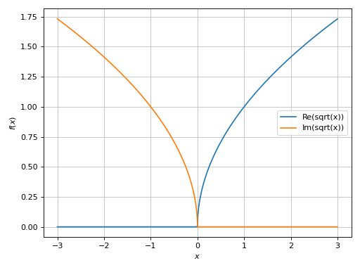
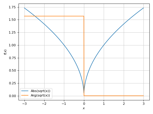
Plot the real and imaginary parts of a function over reals:

>>> plot_real_imag(sqrt(x), (x, -3, 3))
Plot object containing:
[0]: cartesian line: re(sqrt(x)) for x over (-3.0, 3.0)
[1]: cartesian line: im(sqrt(x)) for x over (-3.0, 3.0)

(Source code, png)

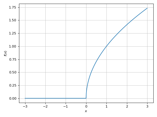
Plot only the real part:

>>> plot_real_imag(sqrt(x), (x, -3, 3), imag=False)
Plot object containing:
[0]: cartesian line: re(sqrt(x)) for x over (-3.0, 3.0)

(Source code, png)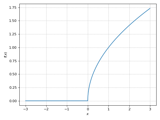

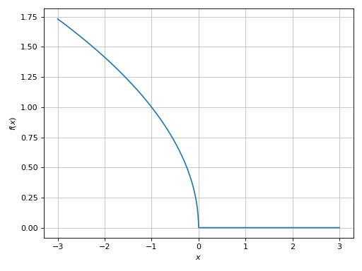
Plot only the imaginary part:

>>> plot_real_imag(sqrt(x), (x, -3, 3), real=False)
Plot object containing:
[0]: cartesian line: im(sqrt(x)) for x over (-3.0, 3.0)

(Source code, png)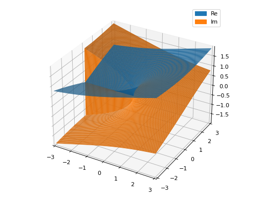

Plot only the absolute value and argument:

>>> plot_real_imag(
...     sqrt(x), (x, -3, 3), real=False, imag=False, abs=True, arg=True)
Plot object containing:
[0]: cartesian line: abs(sqrt(x)) for x over (-3.0, 3.0)
[1]: cartesian line: arg(sqrt(x)) for x over (-3.0, 3.0)

(Source code, png)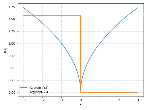

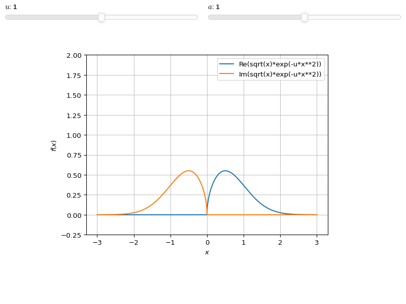
Interactive-widget plot. Refer to the interactive sub-module documentation to learn more about the params dictionary. This plot illustrates:

• the use of prange (parametric plotting range).

• for 1D plot_real_imag, symbols going into prange must be real.

• the use of the params dictionary to specify sliders in their basic form: (default, min, max).

from sympy import *
from spb import *
x, u = symbols("x, u")
a = symbols("a", real=True)
plot_real_imag(sqrt(x) * exp(-u * x**2), prange(x, -3*a, 3*a),
    params={u: (1, 0, 2), a: (1, 0, 2)},
    ylim=(-0.25, 2))

(Source code, small.png)

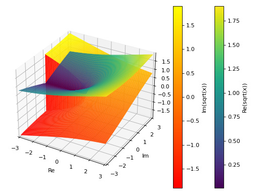
3D plot of the real and imaginary part of the principal branch of a function over a complex range. Note the jump in the imaginary part: that’s a branch cut. The rectangular discretization is unable to properly capture it, hence the near vertical wall. Refer to plot3d_parametric_surface for an example about plotting Riemann surfaces and properly capture the branch cuts.

>>> plot_real_imag(sqrt(x), (x, -3-3j, 3+3j), n=100, threed=True,
...      use_cm=True)
Plot object containing:
[0]: complex cartesian surface: re(sqrt(x)) for re(x) over (-3.0, 3.0) and im(x) over (-3.0, 3.0)
[1]: complex cartesian surface: im(sqrt(x)) for re(x) over (-3.0, 3.0) and im(x) over (-3.0, 3.0)

(Source code, png)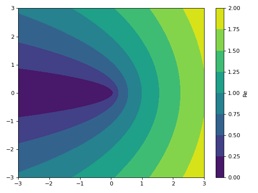

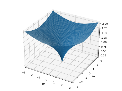
3D plot of the absolute value of a function over a complex range:

>>> plot_real_imag(sqrt(x), (x, -3-3j, 3+3j),
...     n=100, real=False, imag=False, abs=True, threed=True)
Plot object containing:
[0]: complex cartesian surface: abs(sqrt(x)) for re(x) over (-3.0, 3.0) and im(x) over (-3.0, 3.0)

(Source code, png)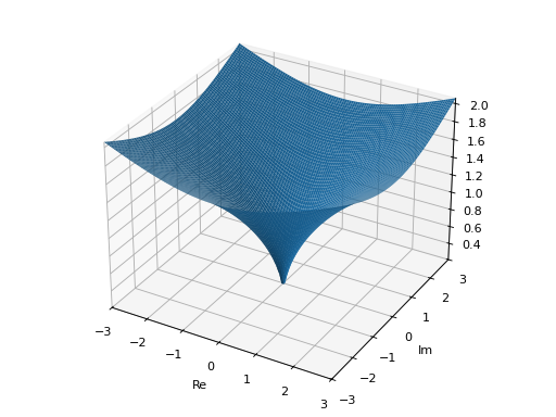

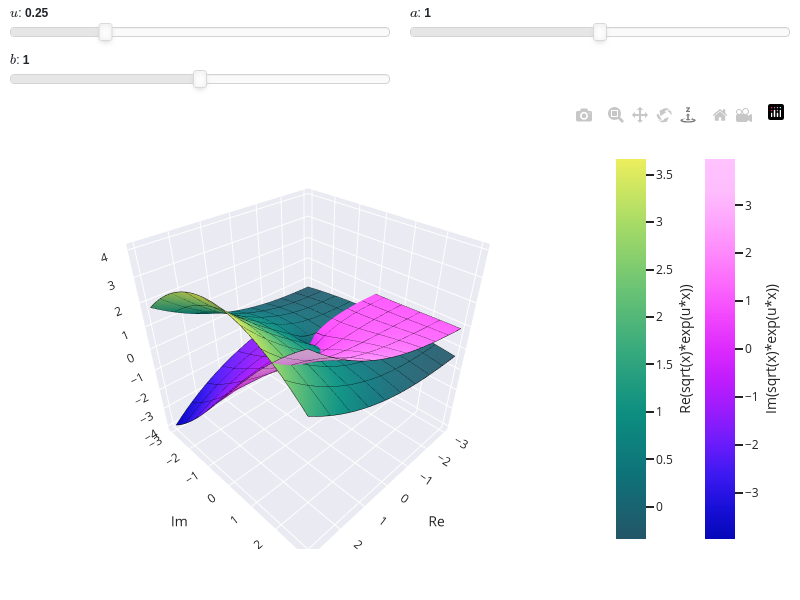
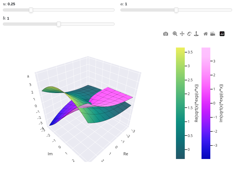
Interactive-widget plot. Refer to the interactive sub-module documentation to learn more about the params dictionary. This plot illustrates:

• the use of prange (parametric plotting range).

• the use of the params dictionary to specify sliders in their basic form: (default, min, max).

from sympy import *
from spb import *
x, u, a, b = symbols("x, u, a, b")
plot_real_imag(
    sqrt(x) * exp(u * x), prange(x, -3*a-b*3j, 3*a+b*3j),
    backend=PB, aspect="cube",
    wireframe=True, wf_rendering_kw={"line_width": 1},
    params={
        u: (0.25, 0, 1),
        a: (1, 0, 2),
        b: (1, 0, 2)
    }, n=25, threed=True, use_cm=True)

(Source code, small.png)

spb.plot_functions.complex_analysis.plot_complex_vector(*args, **kwargs)

Plot the vector field [re(f), im(f)] for a complex function f over the specified complex domain. By default, the aspect ratio of 2D plots is set to aspect="equal".

Typical usage examples are in the followings:

• Plotting a vector field of a complex function:

  plot_complex_vector(expr, range, **kwargs)
  

• Plotting multiple vector fields with different ranges and custom labels:

  plot_complex_vector(
     (expr1, range1, label1 [optional]),
     (expr2, range2, label2 [optional]), **kwargs)
  

Refer to vector_field_2d() for a full list of keyword arguments to customize the appearances of quivers, streamlines and contour.

Refer to graphics() for a full list of keyword arguments to customize the appearances of the figure (title, axis labels, …).

See also

plot_real_imag, plot_complex, plot_complex_list, plot_vector

Examples

>>> from sympy import I, symbols, gamma, latex, log
>>> from spb import plot_complex_vector, plot_complex
>>> z = symbols('z')

(Source code)

Quivers plot with normalize lengths and a contour plot in background representing the vector’s magnitude (a scalar field).

>>> expr = z**2 + 2
>>> plot_complex_vector(expr, (z, -5 - 5j, 5 + 5j),
...     quiver_kw=dict(color="orange"), normalize=True, grid=False)
Plot object containing:
[0]: contour: sqrt(4*(re(_x) - im(_y))**2*(re(_y) + im(_x))**2 + ((re(_x) - im(_y))**2 - (re(_y) + im(_x))**2 + 2)**2) for _x over (-5.0, 5.0) and _y over (-5.0, 5.0)
[1]: 2D vector series: [(re(_x) - im(_y))**2 - (re(_y) + im(_x))**2 + 2, 2*(re(_x) - im(_y))*(re(_y) + im(_x))] over (_x, -5.0, 5.0), (_y, -5.0, 5.0)

(Source code, png)

Only quiver plot with normalized lengths and solid color.

>>> plot_complex_vector(expr, (z, -5 - 5j, 5 + 5j),
...     scalar=False, use_cm=False, normalize=True)
Plot object containing:
[0]: 2D vector series: [(re(_x) - im(_y))**2 - (re(_y) + im(_x))**2 + 2, 2*(re(_x) - im(_y))*(re(_y) + im(_x))] over (_x, -5.0, 5.0), (_y, -5.0, 5.0)

(Source code, png)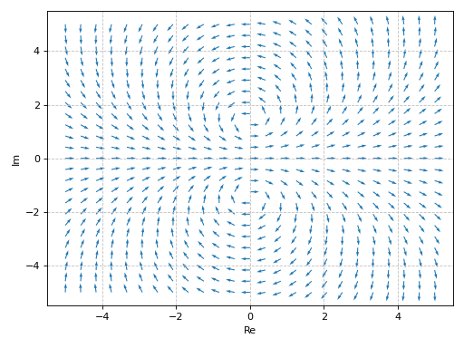

Only streamlines plot.

>>> plot_complex_vector(expr, (z, -5 - 5j, 5 + 5j),
...     "Magnitude of $%s$" % latex(expr),
...     scalar=False, streamlines=True)
Plot object containing:
[0]: 2D vector series: [(re(_x) - im(_y))**2 - (re(_y) + im(_x))**2 + 2, 2*(re(_x) - im(_y))*(re(_y) + im(_x))] over (_x, -5.0, 5.0), (_y, -5.0, 5.0)

(Source code, png)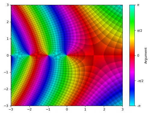

Overlay the quiver plot to a domain coloring plot. By setting n=26 (even number) in the complex vector plot, the quivers won’t to cross the branch cut.

>>> expr = z * log(2 * z) + 3
>>> p1 = plot_complex(expr, (z, -2-2j, 2+2j), grid=False, show=False,
...     legend=False)
>>> p2 = plot_complex_vector(expr, (z, -2-2j, 2+2j),
...      n=26, grid=False, scalar=False, use_cm=False, normalize=True,
...      quiver_kw={"color": "k", "pivot": "tip"}, show=False)
>>> (p1 + p2).show()
>>> (p1 + p2)
Plot object containing:
[0]: complex domain coloring: z*log(2*z) + 3 for re(z) over (-2.0, 2.0) and im(z) over (-2.0, 2.0)
[1]: 2D vector series: [(re(_x) - im(_y))*log(Abs(2*_x + 2*_y*I)) - (re(_y) + im(_x))*arg(_x + _y*I) + 3, (re(_x) - im(_y))*arg(_x + _y*I) + (re(_y) + im(_x))*log(Abs(2*_x + 2*_y*I))] over (_x, -2.0, 2.0), (_y, -2.0, 2.0)

(Source code, png)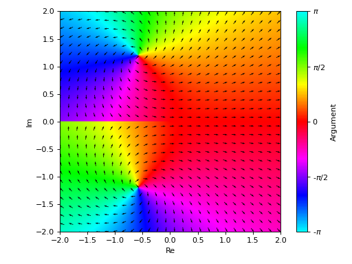

Interactive-widget plot. Refer to the interactive sub-module documentation to learn more about the params dictionary. This plot illustrates:

• the use of prange (parametric plotting range).

• the use of the params dictionary to specify sliders in their basic form: (default, min, max).

from sympy import *
from spb import *
z, u, a, b = symbols("z u a b")
plot_complex_vector(
    log(gamma(u * z)), prange(z, -5*a - b*5j, 5*a + b*5j),
    params={
        u: (1, 0, 2),
        a: (1, 0, 2),
        b: (1, 0, 2)
    }, n=20, grid=False,
    quiver_kw=dict(color="orange", headwidth=4))

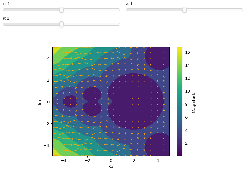
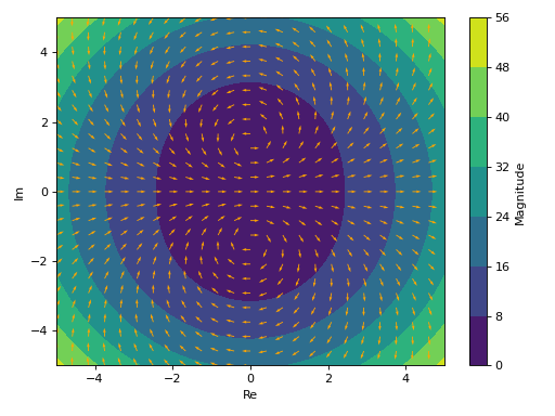
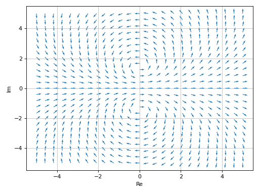
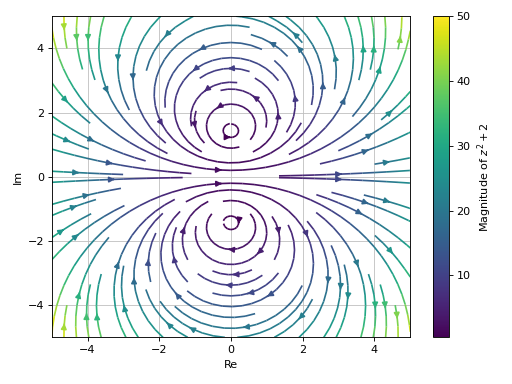
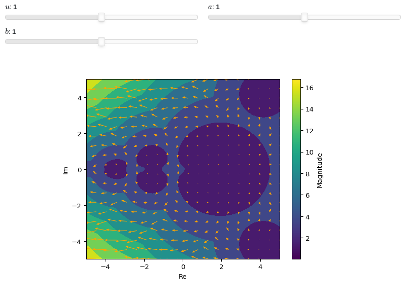(Source code, small.png)